Implementing SummAE neural text summarization with a denoising auto-encoder

By Kamil Ciemniewski
May 28, 2020

If there’s any problem space in machine learning, with no shortage of (unlabelled) data to train on, it’s easily natural language processing (NLP).
In this article, I’d like to take on the challenge of taking a paper that came from Google Research in late 2019 and implementing it. It’s going to be a fun trip into the world of neural text summarization. We’re going to go through the basics, the coding, and then we’ll look at what the results actually are in the end.
The paper we’re going to implement here is: Peter J. Liu, Yu-An Chung, Jie Ren (2019) SummAE: Zero-Shot Abstractive Text Summarization using Length-Agnostic Auto-Encoders.
Here’s the paper’s abstract:
We propose an end-to-end neural model for zero-shot abstractive text summarization of paragraphs, and introduce a benchmark task, ROCSumm, based on ROCStories, a subset for which we collected human summaries. In this task, five-sentence stories (paragraphs) are summarized with one sentence, using human summaries only for evaluation. We show results for extractive and human baselines to demonstrate a large abstractive gap in performance. Our model, SummAE, consists of a denoising auto-encoder that embeds sentences and paragraphs in a common space, from which either can be decoded. Summaries for paragraphs are generated by decoding a sentence from the paragraph representations. We find that traditional sequence-to-sequence auto-encoders fail to produce good summaries and describe how specific architectural choices and pre-training techniques can significantly improve performance, outperforming extractive baselines. The data, training, evaluation code, and best model weights are open-sourced.
Preliminaries
Before we go any further, let’s talk a little bit about neural summarization in general. There’re two main approaches to it:
The first approach makes the model “focus” on the most important parts of the longer text - extracting them to form a summary.
Let’s take a recent article, “Shopify Admin API: Importing Products in Bulk”, by one of my great co-workers, Patrick Lewis, as an example and see what the extractive summarization would look like. Let’s take the first two paragraphs:
I recently worked on an interesting project for a store owner who was facing a daunting task: he had an inventory of hundreds of thousands of Magic: The Gathering (MTG) cards that he wanted to sell online through his Shopify store. The logistics of tracking down artwork and current market pricing for each card made it impossible to do manually.
My solution was to create a custom Rails application that retrieves inventory data from a combination of APIs and then automatically creates products for each card in Shopify. The resulting project turned what would have been a months- or years-long task into a bulk upload that only took a few hours to complete and allowed the store owner to immediately start selling his inventory online. The online store launch turned out to be even more important than initially expected due to current closures of physical stores.
An extractive model could summarize it as follows:
I recently worked on an interesting project for a store owner who had an inventory of hundreds of thousands of cards that he wanted to sell through his store. The logistics and current pricing for each card made it impossible to do manually. My solution was to create a custom Rails application that retrieves inventory data from a combination of APIs and then automatically creates products for each card. The store launch turned out to be even more important than expected due to current closures of physical stores.
See how it does the copying and pasting? The big advantage of these types of models is that they are generally easier to create and the resulting summaries tend to faithfully reflect the facts included in the source.
The downside though is that it’s not how a human would do it. We do a lot of paraphrasing, for instance. We use different words and tend to form sentences less rigidly following the original ones. The need for the summaries to feel more natural made the second type — abstractive — into this subfield’s holy grail.
Datasets
The paper’s authors used the so-called “ROCStories” dataset (“Tackling The Story Ending Biases in The Story Cloze Test”. Rishi Sharma, James Allen, Omid Bakhshandeh, Nasrin Mostafazadeh. In Proceedings of the 2018 Conference of the Association for Computational Linguistics (ACL), 2018).
In my experiments, I’ve also tried the model against one that’s quite a bit more difficult: WikiHow (Mahnaz Koupaee, William Yang Wang (2018) WikiHow: A Large Scale Text Summarization Dataset).
ROCStories
The dataset consists of 98162 stories, each one consisting of 5 sentences. It’s incredibly clean. The only step I needed to take was to split the stories between the train, eval, and test sets.
Examples of sentences:
Example 1:
My retired coworker turned 69 in July. I went net surfing to get her a gift. She loves Diana Ross. I got two newly released cds and mailed them to her. She sent me an email thanking me.
Example 2:
Tom alerted the government he expected a guest. When she didn’t come he got in a lot of trouble. They talked about revoking his doctor’s license. And charging him a huge fee! Tom’s life was destroyed because of his act of kindness.
Example 3:
I went to see the doctor when I knew it was bad. I hadn’t eaten in nearly a week. I told him I felt afraid of food in my body. He told me I was developing an eating disorder. He instructed me to get some help.
Wikihow
This is one of the most challenging openly available datasets for neural summarization. It consists of more than 200,000 long-sequence pairs of text + headline scraped from WikiHow’s website.
Some examples:
Text:
One easy way to conserve water is to cut down on your shower time. Practice cutting your showers down to 10 minutes, then 7, then 5. Challenge yourself to take a shorter shower every day. Washing machines take up a lot of water and electricity, so running a cycle for a couple of articles of clothing is inefficient. Hold off on laundry until you can fill the machine. Avoid letting the water run while you’re brushing your teeth or shaving. Keep your hoses and faucets turned off as much as possible. When you need them, use them sparingly.
Headline:
Take quicker showers to conserve water. Wait for a full load of clothing before running a washing machine. Turn off the water when you’re not using it.
The main challenge for the summarization model here is that the headline was actually created by humans and is not just “extracting” anything. Any model performing well on this dataset actually needs to model the language pretty well. Otherwise, the headline could be used for computing the evaluation metrics, but it’s pretty clear that traditional metrics like ROUGE are just bound here to miss the point.
Basics of the sequence-to-sequence modeling
Most sequence-to-sequence models are based on the “next token prediction” workflow.
The general idea can be expressed with P(token | context) — where the task is to model this conditional probability distribution. The “context” here depends on the approach.
Those models are also called “auto-regressive” because they need to consume their own predictions from previous steps during the inference:
predict(["<start>"], context)
# "I"
predict(["<start>", "I"], context)
# "love"
predict(["<start>", "I", "love"], context)
# "biking"
predict(["<start>", "I", "love", "biking"], context)
# "<end>"
Naively simple modeling: Markov Model
In this model, the approach is to take on a bold assumption: that the probability of the next token is conditioned only on the previous token.
The Markov Model is elegantly introduced in the blog post Next Word Prediction using Markov Model.
Why is it naive? Because we know that the probability of the word “love” depends on the word “I” given a broader context. A model that’s always going to output “roses” would miss the best word more often than not.
Modeling with neural networks
Usually, sequence-to-sequence neural network models consist of two parts:
- encoder
- decoder
The encoder is there to build a “gist” representation of the input sequence. The gist and the previous token become our “context” to do the inference. This fits in well within the P(token | context) modeling I described above. That distribution can be expressed more clearly as P(token | previous; gist).
There are other approaches too with one of them being the ProphetNet: Predicting Future N-gram for Sequence-to-Sequence Pre-training - 2020 - Yan, Yu and Qi, Weizhen and Gong, Yeyun and Liu, Dayiheng and Duan, Nan and Chen, Jiusheng and Zhang, Ruofei and Zhou, Ming. The difference in the approach here was the prediction of n-tokens ahead at once.
Teacher-forcing
Let’s see how could we go about teaching the model about the next token’s conditional distribution.
Imagine that the model’s parameters aren’t performing well yet. We have an input sequence of: ["<start>", "I", "love", "biking", "during", "the", "summer", "<end>"]. We’re training the model giving it the first token:
model(["<start>", context])
# "I"
Great, now let’s ask it for another one:
model(["<start>", "I"], context])
# "wonder"
Hmmm that’s not what we wanted, but let’s naively continue:
model(["<start>", "I", "wonder"], context)
# "why"
We could continue gathering predictions and compute the loss at the end. The loss would really only be able to tell it about the first mistake (“love” vs. “wonder”); the rest of the errors would just accumulate from here. This would hinder the learning considerably, adding in the noise from the accumulated errors.
There’s a better approach called Teacher Forcing. In this approach, you’re telling the model the true answer after each of its guesses. The last example would look like the following:
model(["<start>", "I", "love"], context)
# "watching"
You’d continue the process, feeding it the full input sequence and the loss term would be computed based on all its guesses.
Compute-friendly representation for tokens and gists
Some of the readers might want to skip this section. I’d like to describe quickly here the concept of the latent space and vector embeddings. This is to keep the matters relatively palatable for the broader audience.
Representing words naively
How do we turn the words (strings) into numbers that we input into our machine learning models? A software developer might think about assigning each word a unique integer. This works well for databases but in machine learning models, the fact that integers follow one another means that they encode a relation (which one follows which and in what distance). This doesn’t work well for almost any problem in data science.
Traditionally, the problem is solved by “one-hot encoding”. This means that we’re turning our integers into vectors, where each value is zero except the one for the index that equals the value to encode (or minus one if your programming language uses zero-based indexing). Example: 3 => [0, 0, 0, 1, 0, 0, 0, 0, 0, 0] when the total number of “integers” (classes) to encode is 10.
This is better as it breaks the ordering and distancing assumptions. It doesn’t encode anything about the words, though, except the arbitrary number we’ve decided to assign to them. We now don’t have the ordering but we also don’t have any distance. Empirically though we just know that the word “love” is much closer to “enjoy” than it is to “helicopter”.
A better approach: word embeddings
How could we keep our vector representation (as in one-hot encoding) but also introduce the distance? I’ve already glanced over this concept in my post about the simple recommender system. The idea is to have a vector of floating-point values so that the closer the words are in their meaning, the smaller the angle is between them. We can easily compute a metric following this logic by measuring the cosine distance. This way, the word representations are easy to feed into the encoder, and they already contain a lot of the information in themselves.
Not only words
Can we only have vectors for words? Couldn’t we have vectors for paragraphs, so that the closer they are in their meaning, the smaller some vector space metric between them? Of course we can. This is, in fact, what will allow us in this article’s model to encode the “gist” that we talked about. The “encoder” part of the model is going to learn the most convenient way of turning the input sequence into the floating-point numbers vector.
Auto-encoders
We’re slowly approaching the model from the paper. We still have one concept that’s vital to understand in order to get why the model is going to work.
Up until now, we talked about the following structure of the typical sequence-to-sequence neural network model:
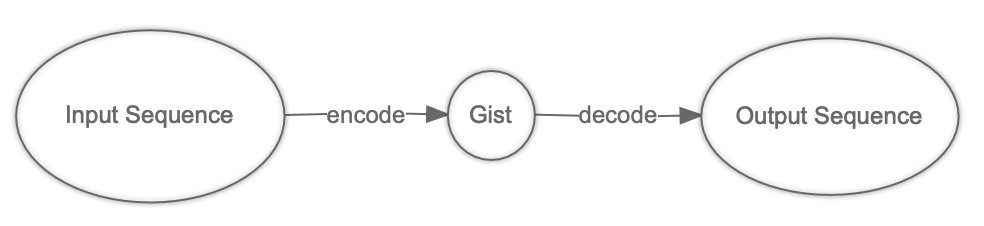
This is true e.g. for translation models where the input sequence is in English and the output is in Greek. It’s also true for this article’s model during the inference.
What if we’d make the input and output to be the same sequence? We’d turn it into a so-called auto-encoder.
The output of course isn’t all that useful — we already know what the input sequence is. The true value is in the model’s ability to encode the input into a gist.
Adding the noise
A very interesting type of an auto-encoder is the denoising auto-encoder. The idea is that the input sequence gets randomly corrupted and the network learns to still produce a good gist and reconstruct the sequence before it got corrupted. This makes the training “teach” the network about the deeper connections in the data, instead of just “memorizing” as much as it can.
The SummAE model
We’re now ready to talk about the architecture from the paper. Given what we’ve already learned, this is going to be very simple. The SummAE model is just a denoising auto-encoder that is being trained a special way.
Auto-encoding paragraphs and sentences
The authors were training the model on both single sentences and full paragraphs. In all cases the task was to reproduce the uncorrupted input.
The first part of the approach is about having two special “start tokens” to signal the mode: paragraph vs. sentence. In my code, I’ve used “<start-full>” and “<start-short>”.
During the training, the model learns the conditional distributions given those two tokens and the ones that follow, for any given token in the sequence.
Adding the noise
The sentences are simply concatenated to form a paragraph. The input then gets corrupted at random by means of:
- masking the input tokens
- shuffling the order of the sentences within the paragraph
The authors are claiming that the latter helped them in solving the issue of the network just memorizing the first sentence. What I have found though is that this model is generally prone towards memorizing concrete sentences from the paragraph. Sometimes it’s the first, and sometimes it’s some of the others. I’ve found this true even when adding a lot of noise to the input.
The code
The full PyTorch implementation described in this blog post is available at https://github.com/kamilc/neural-text-summarization. You may find some of its parts less clean than others — it’s a work in progress. Specifically, the data download is almost left out.
You can find the WikiData preprocessing in a notebook in the repository. For the ROCStories, I just downloaded the CSV files and concatenated with Unix cat. There’s an additional process.py file generated from a very simple IPython session.
Let’s have a very brief look at some of the most interesting parts of the code:
class SummarizeNet(NNModel):
    def encode(self, embeddings, lengths):
        # ...

    def decode(self, embeddings, encoded, lengths, modes):
        # ...

    def forward(self, embeddings, clean_embeddings, lengths, modes):
        # ...

    def predict(self, vocabulary, embeddings, lengths):
        # ...
You can notice separate methods for forward and predict. I chose the Transformer over the recurrent neural networks for both the encoder part and the decoder. The PyTorch implementation of the transformer decoder part already includes the teacher forcing in the forward method. This makes it convenient at the training time — to just feed it the full, uncorrupted sequence of embeddings as the “target”. During the inference we need to do the “auto-regressive” part by hand though. This means feeding the previous predictions in a loop — hence the need for two distinct methods here.
def forward(self, embeddings, clean_embeddings, lengths, modes):
    noisy_embeddings = self.mask_dropout(embeddings, lengths)

    encoded = self.encode(noisy_embeddings[:, 1:, :], lengths-1)
    decoded = self.decode(clean_embeddings, encoded, lengths, modes)

    return (
        decoded,
        encoded
    )
You can notice that I’m doing the token masking at the model level during the training. The code also shows cleanly the structure of this seq2seq model — with the encoder and the decoder.
The encoder part looks simple as long as you’re familiar with the transformers:
def encode(self, embeddings, lengths):
    batch_size, seq_len, _ = embeddings.shape

    embeddings = self.encode_positions(embeddings)

    paddings_mask = torch.arange(end=seq_len).unsqueeze(dim=0).expand((batch_size, seq_len)).to(self.device)
    paddings_mask = (paddings_mask + 1) > lengths.unsqueeze(dim=1).expand((batch_size, seq_len))

    encoded = embeddings.transpose(1,0)

    for ix, encoder in enumerate(self.encoders):
        encoded = encoder(encoded, src_key_padding_mask=paddings_mask)
        encoded = self.encode_batch_norms[ix](encoded.transpose(2,1)).transpose(2,1)

    last_encoded = encoded

    encoded = self.pool_encoded(encoded, lengths)

    encoded = self.to_hidden(encoded)

    return encoded
We’re first encoding the positions as in the “Attention Is All You Need” paper and then feeding the embeddings into a stack of the encoder layers. At the end, we’re morphing the tensor to have the final dimension equal the number given as the model’s parameter.
The decode sits on PyTorch’s shoulders too:
def decode(self, embeddings, encoded, lengths, modes):
    batch_size, seq_len, _ = embeddings.shape

    embeddings = self.encode_positions(embeddings)

    mask = self.mask_for(embeddings)

    encoded = self.from_hidden(encoded)
    encoded = encoded.unsqueeze(dim=0).expand(seq_len, batch_size, -1)

    decoded = embeddings.transpose(1,0)
    decoded = torch.cat(
        [
            encoded,
            decoded
        ],
        axis=2
    )
    decoded = self.combine_decoded(decoded)
    decoded = self.combine_batch_norm(decoded.transpose(2,1)).transpose(2,1)

    paddings_mask = torch.arange(end=seq_len).unsqueeze(dim=0).expand((batch_size, seq_len)).to(self.device)
    paddings_mask = paddings_mask > lengths.unsqueeze(dim=1).expand((batch_size, seq_len))

    for ix, decoder in enumerate(self.decoders):
        decoded = decoder(
            decoded,
            torch.ones_like(decoded),
            tgt_mask=mask,
            tgt_key_padding_mask=paddings_mask
        )
        decoded = self.decode_batch_norms[ix](decoded.transpose(2,1)).transpose(2,1)

    decoded = decoded.transpose(1,0)

    return self.linear_logits(decoded)
You can notice that I’m combining the gist received from the encoder with each word embeddings — as this is how it was described in the paper.
The predict is very similar to forward:
def predict(self, vocabulary, embeddings, lengths):
    """
    Caller should include the start and end tokens here
    but we’re going to ensure the start one is replaces by <start-short>
    """
    previous_mode = self.training

    self.eval()

    batch_size, _, _ = embeddings.shape

    results = []

    for row in range(0, batch_size):
        row_embeddings = embeddings[row, :, :].unsqueeze(dim=0)
        row_embeddings[0, 0] = vocabulary.token_vector("<start-short>")

        encoded = self.encode(
            row_embeddings[:, 1:, :],
            lengths[row].unsqueeze(dim=0)
        )

        results.append(
            self.decode_prediction(
                vocabulary,
                encoded,
                lengths[row].unsqueeze(dim=0)
            )
        )

    self.training = previous_mode

    return results
The workhorse behind the decoding at the inference time looks as follows:
def decode_prediction(self, vocabulary, encoded1xH, lengths1x):
    tokens = ['<start-short>']
    last_token = None
    seq_len = 1

    encoded1xH = self.from_hidden(encoded1xH)

    while last_token != '<end>' and seq_len < 50:
        embeddings1xSxD = vocabulary.embed(tokens).unsqueeze(dim=0).to(self.device)
        embeddings1xSxD = self.encode_positions(embeddings1xSxD)

        maskSxS = self.mask_for(embeddings1xSxD)

        encodedSx1xH = encoded1xH.unsqueeze(dim=0).expand(seq_len, 1, -1)

        decodedSx1xD = embeddings1xSxD.transpose(1,0)
        decodedSx1xD = torch.cat(
            [
                encodedSx1xH,
                decodedSx1xD
            ],
            axis=2
        )
        decodedSx1xD = self.combine_decoded(decodedSx1xD)
        decodedSx1xD = self.combine_batch_norm(decodedSx1xD.transpose(2,1)).transpose(2,1)

        for ix, decoder in enumerate(self.decoders):
            decodedSx1xD = decoder(
                decodedSx1xD,
                torch.ones_like(decodedSx1xD),
                tgt_mask=maskSxS,
            )
            decodedSx1xD = self.decode_batch_norms[ix](decodedSx1xD.transpose(2,1))
            decodedSx1xD = decodedSx1xD.transpose(2,1)

        decoded1x1xD = decodedSx1xD.transpose(1,0)[:, (seq_len-1):seq_len, :]
        decoded1x1xV = self.linear_logits(decoded1x1xD)

        word_id = F.softmax(decoded1x1xV[0, 0, :]).argmax().cpu().item()
        last_token = vocabulary.words[word_id]
        tokens.append(last_token)
        seq_len += 1

    return ' '.join(tokens[1:])
You can notice starting with the “start short” token and going in a loop, getting predictions, and feeding back until the “end” token.
Again, the model is very, very simple. What makes the difference is how it’s being trained — it’s all in the training data corruption and the model pre-training.
It’s already a long article so I encourage the curious readers to look at the code at my GitHub repo for more details.
My experiment with the WikiHow dataset
In my WikiHow experiment I wanted to see how the results look if I fed the full articles and their headlines for the two modes of the network. The same data-corruption regime was used in this case.
Some of the results were looking almost good:
Text:
for a savory flavor, mix in 1/2 teaspoon ground cumin, ground turmeric, or masala powder.this works best when added to the traditional salty lassi. for a flavorful addition to the traditional sweet lassi, add 1/2 teaspoon of ground cardamom powder or ginger, for some kick. , start with a traditional sweet lassi and blend in some of your favorite fruits. consider mixing in strawberries, papaya, bananas, or coconut.try chopping and freezing the fruit before blending it into the lassi. this will make your drink colder and frothier. , while most lassi drinks are yogurt based, you can swap out the yogurt and water or milk for coconut milk. this will give a slightly tropical flavor to the drink. or you could flavor the lassi with rose water syrup, vanilla extract, or honey.don’t choose too many flavors or they could make the drink too sweet. if you stick to one or two flavors, they’ll be more pronounced. , top your lassi with any of the following for extra flavor and a more polished look: chopped pistachios sprigs of mint sprinkle of turmeric or cumin chopped almonds fruit sliver
Headline:
add a spice., blend in a fruit., flavor with a syrup or milk., garnish.
Predicted summary:
blend vanilla in a sweeter flavor . , add a sugary fruit . , do a spicy twist . eat with dessert . , revise .
It’s not 100% faithful to the original text even though it seems to “read” well.
My suspicion is that pre-training against a much larger corpus of text might possibly help. There’s an obvious issue with the lack of very specific knowledge here to have the network summarize better. Here’s another of those examples:
Text:
the settings app looks like a gray gear icon on your iphone’s home screen.; , this option is listed next to a blue “a” icon below general. , this option will be at the bottom of the display & brightness menu. , the right-hand side of the slider will give you bigger font size in all menus and apps that support dynamic type, including the mail app. you can preview the corresponding text size by looking at the menu texts located above and below the text size slider. , the left-hand side of the slider will make all dynamic type text smaller, including all menus and mailboxes in the mail app. , tap the back button twice in the upper-left corner of your screen. it will save your text size settings and take you back to your settings menu. , this option is listed next to a gray gear icon above display & brightness. , it’s halfway through the general menu. ,, the switch will turn green. the text size slider below the switch will allow for even bigger fonts. , the text size in all menus and apps that support dynamic type will increase as you go towards the right-hand side of the slider. this is the largest text size you can get on an iphone. , it will save your settings.
Headline:
open your iphone’s settings., scroll down and tap display & brightness., tap text size., tap and drag the slider to the right for bigger text., tap and drag the slider to the left for smaller text., go back to the settings menu., tap general., tap accessibility., tap larger text. , slide the larger accessibility sizes switch to on position., tap and drag the slider to the right., tap the back button in the upper-left corner.
Predicted summary:
open your iphone ’s settings . , tap general . , scroll down and tap accessibility . , tap larger accessibility . , tap and larger text for the iphone to highlight the text you want to close . , tap the larger text - colored contacts app .
It might be interesting to train against this dataset again while:
- utilizing some pre-trained, large scale model as part of the encoder
- using a large corpus of text to still pre-train the auto-encoder
This could possibly take a lot of time to train on my GPU (even with the pre-trained part of the encoder). I didn’t follow the idea further at this time.
The problem with getting paragraphs when we want the sentences
One of the biggest problems the authors ran into was with the decoder outputting the long version of the text, even though it was asked for the sentence-long summary.
Authors called this phenomenon the “segregation issue”. What they have found was that the encoder was mapping paragraphs and sentences into completely separate regions. The solution to this problem was to trick the encoder into making both representations indistinguishable. The following figure comes from the paper and shows the issue visualized:
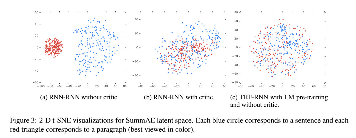
Better gists by using the “critic”
The idea of a “critic” has been popularized along with the fantastic results produced by some of the Generative Adversarial Networks. The general workflow is to have the main network generate output while the other tries to guess some of its properties.
For GANs that are generating realistic photos, the critic is there to guess if the photo was generated or if it’s real. A loss term is added based on how well it’s doing, penalizing the main network for generating photos that the critic is able to call out as fake.
A similar idea was used in the A3C algorithm I blogged about (Self-driving toy car using the Asynchronous Advantage Actor-Critic algorithm). The “critic” part penalized the AI agent for taking steps that were on average less advantageous.
Here, in the SummAE model, the critic adds a penalty to the loss to the degree to which it’s able to guess whether the gist comes from a paragraph or a sentence.
Training with the critic might get tricky. What I’ve found to be the cleanest way is to use two different optimizers — one updating the main network’s parameters while the other updates the critic itself:
for batch in batches:
    if mode == "train":
        self.model.train()
        self.discriminator.train()
    else:
        self.model.eval()
        self.discriminator.eval()

    self.optimizer.zero_grad()
    self.discriminator_optimizer.zero_grad()

    logits, state = self.model(
        batch.word_embeddings.to(self.device),
        batch.clean_word_embeddings.to(self.device),
        batch.lengths.to(self.device),
        batch.mode.to(self.device)
    )

    mode_probs_disc = self.discriminator(state.detach())
    mode_probs = self.discriminator(state)

    discriminator_loss = F.binary_cross_entropy(
        mode_probs_disc,
        batch.mode
    )

    discriminator_loss.backward(retain_graph=True)

    if mode == "train":
        self.discriminator_optimizer.step()

    text = batch.text.copy()

    if self.no_period_trick:
        text = [txt.replace('.', '') for txt in text]

    classes = self.vocabulary.encode(text, modes=batch.mode)
    classes = classes.roll(-1, dims=1)
    classes[:,classes.shape[1]-1] = 3

    model_loss = torch.tensor(0).cuda()

    if logits.shape[0:2] == classes.shape:
        model_loss = F.cross_entropy(
            logits.reshape(-1, logits.shape[2]).to(self.device),
            classes.long().reshape(-1).to(self.device),
            ignore_index=3
        )
    else:
        print("WARNING: Skipping model loss for inconsistency between logits and classes shapes")

    fooling_loss = F.binary_cross_entropy(
        mode_probs,
        torch.ones_like(batch.mode).to(self.device)
    )

    loss = model_loss + (0.1 * fooling_loss)

    loss.backward()
    if mode == "train":
        self.optimizer.step()

    self.optimizer.zero_grad()
    self.discriminator_optimizer.zero_grad()
The main idea is to treat the main network’s encoded gist as constant with respect to the updates to the critic’s parameters, and vice versa.
Results
I’ve found some of the results look really exceptional:
Text:
lynn is unhappy in her marriage. her husband is never good to her and shows her no attention. one evening lynn tells her husband she is going out with her friends. she really goes out with a man from work and has a great time. lynn continues dating him and starts having an affair.
Predicted summary:
lynn starts dating him and has an affair .
Text:
cedric was hoping to get a big bonus at work. he had worked hard at the office all year. cedric’s boss called him into his office. cedric was disappointed when told there would be no bonus. cedric’s boss surprised cedric with a big raise instead of a bonus.
Predicted summary:
cedric had a big deal at his boss ’s office .
Some others showed how the model attends to single sentences though:
Text:
i lost my job. i was having trouble affording my necessities. i didn’t have enough money to pay rent. i searched online for money making opportunities. i discovered amazon mechanical turk.
Predicted summary:
i did n’t have enough money to pay rent .
While the sentence like this one would maybe make a good headline — it’s definitely not the best summary as it naturally loses the vital parts found in other sentences.
Final words
First of all, let me thank the paper’s authors for their exceptional work. It was a great read and great fun implementing!
Abstractive text summarization remains very difficult. The model trained for this blog post has very limited use in practice. There’s a lot of room for improvement though, which makes the future of abstractive summaries very promising.
python machine-learning artificial-intelligence natural-language-processing
Comments