Our Blog

Building Rasters in PostGIS

By Josh Tolley
September 12, 2018

In a past blog post I described a method I’d used to digest raw statistics from the Mexican government statistics body, INEGI, quantifying the relative educational level of residents in Mexico City. In the post, I divided these data into squares geographically, and created a KML visualization consisting of polygons, where each polygon’s color and height reflected the educational level of residents in the corresponding area. Where the original data proved slow to render and difficult to interpret, the result after processing was visually appealing, intuitively meaningful, and considerably more performant. Plus I got to revisit a favorite TV show, examine SQL’s Common Table Expressions, and demonstrate their use in building complex queries.

But the post left a few loose ends untied. For instance, the blog post built the visualization using just one large query. Although its CTE-based design rendered it fairly readable, the query remained far too complex, and far too slow, at least for general use. Doing everything in one query makes for a sometimes enjoyable mental exercise, but it also means the query has to start from zero, every time it runs, so iterative development bogs down quickly as the query must recalculate at every new iteration all the expensive stuff it already got worked out in previous runs. Further, the query in that post calculated its grid coordinates all on its own; there’s an easier method I promised to introduce, which I’d like to demonstrate here.

Rasters

GIS databases contain information of (at least) two different types: vector data, and raster data. Vector data describes points, connected with lines and curves, and various objects derived from them, such as polygons and linestrings. Rasters, on the other hand, represent a two dimensional array of pixels, where each pixel corresponds to a certain geographic area. Each pixel in the raster will have two sets of associated coordinates: first, latitude and longitude values describing the geographic square this pixel represents, and second, the pixel coordinates within the raster, which in PostGIS begin with (1,1) at the origin. Rasters organize their data in “bands”, collections of boolean or numeric values, with at most one value per pixel. One band might represent the elevation above sea level for each pixel, or the surface temperature. Aerial imagery is often delivered as rasters: a full-color image might have one band for the red channel, another for green, and a third for blue. Bands may also contain no value for certain pixels, and we’ll make use of this ability later to make some parts of our final image transparent.

The Data

The INEGI data I introduced in my previous blog post contains points representing every school in Mexico, and continuing on the theme of education, I thought it would be an interesting exercise to make an image of the country, where the color varies depending on the concentration of schools in the area. This resembles my previous work in many ways: I’m dividing the area under consideration into small parts, generating a value for each of those parts, and representing the result visually. Here, though, rather than drawing and extruding polygons, I’ll simply color a raster pixel. This simpler rendering, where the display system must simply project a static image, rather than an array of polygons, means I can support a much higher resolution grid than in my previous blog post, without overtaxing display hardware.

Creating the Image

Having learned my lesson from the work with Mexico City data, I elected to create this image with multiple queries. In the end, I wrapped these queries in a Perl script, building sufficient intelligence therein to recreate any bits of the database I might have simply dropped, as I developed the script, and to skip reprocessing any steps for which it finds current results lying around.

PostGIS supports a data type called raster, and anticipating that I might want multiple rasters in my database each using a variety of settings and script modifications, I created a table to store these rasters and some extra data about them.

CREATE TABLE rasters (id SERIAL PRIMARY KEY, pixels INTEGER, r RASTER, comment TEXT);

The pixels field holds the number of pixels along one edge of the raster, which the script presumes is a square. This is redundant, as I can extract that number from the raster itself, but having it stored here made things easier for my purposes.

To calculate a raster, I need to find a value for each of its pixels, or to confirm that the pixel should have no value, and for that I wanted another table. This table contains both geographic and Euclidean coordinates for each pixel in each raster, the id of the associated entry in the rasters table, a field for the number of schools I’ve counted in this square, fields for the RGB color assigned to the pixel, and a boolean flag telling me whether or not I’ve finished calculating everything for this pixel or not.

CREATE TABLE polys (
    x INTEGER,
    y INTEGER,
    geom GEOMETRY,
    count INTEGER,
    r_val INTEGER,
    b_val INTEGER,
    g_val INTEGER,
    processed BOOLEAN DEFAULT 'f',
    raster_id INTEGER NOT NULL
);

The script’s first step is to create an empty raster, which it does with PostGIS’s ST_MakeEmptyRaster() function, and to add four bands to it, one each for the pixels’ red, green, blue, and alpha values. The data type for each band is given as 8BUI, PostGIS parlance for an 8-bit unsigned integer. The various color bands default to NULL values, and the alpha band to zeroes. The code looks something like this:

INSERT INTO rasters (pixels, r, comment)
SELECT
    ST_AddBand(
    ST_AddBand(
    ST_AddBand(
    ST_AddBand(
        ST_MakeEmptyRaster(
            numpixels,  -- The number of pixels along one edge of the raster
            numpixels,
            st_xmin,    -- latitude and longitude coordinates of the corner of the raster
            st_ymax,
            (st_xmax - st_xmin)/numpixels::float,   -- width and height of the raster
            -(st_ymax - st_ymin)/numpixels::float,
            0,
            0,
            4326        -- We'll use the WGS 84 coordinate system
        ),
        1, '8BUI'::TEXT, NULL::DOUBLE PRECISION, NULL::DOUBLE PRECISION),
        2, '8BUI'::TEXT, NULL::DOUBLE PRECISION, NULL::DOUBLE PRECISION),
        3, '8BUI'::TEXT, NULL::DOUBLE PRECISION, NULL::DOUBLE PRECISION),
        4, '8BUI'::TEXT, 0, 0
    ) AS r
FROM limits, params;

The query refers to the limits and params tables (actually, they’re table expressions from elsewhere in the query from which this snippet is extracted). These tables provide values for numpixels, the number of pixels along one edge of the raster, provided by the user on the script’s command line, and for st_xmin, st_xmax, st_ymin, and st_ymax, which are latitude and longitude values describing a bounding box around the Mexican territory.

Before we can do too much experimentation and query development, we need a way to inspect our results, by rendering the raster from the database to an actual image file. This is one place where having a Perl wrapper script comes in handy, because doing this in pure SQL is actually something of a pain..

print "Creating image\n";
my $res = $dbh->selectall_arrayref(qq{
    SELECT ST_AsPng(r, ARRAY[1,2,3,4]::INT[])
    FROM rasters WHERE id = $id
});

my $png = $res->[0][0];

open (my $fh, '>', $filename) || die "Couldn't open handle to $filename: $!";
binmode $fh;

print $fh $png;

close $fh;

This uses ST_AsPng to create an image file under whatever path is stored in $filename, and it’s helpful for reviewing incremental results as the script develops, and of course for rendering the final product. Here we’ve told it to use band 1 for the red values, band 2 for green, 3 for blue, and 4 for alpha. The alpha channel is important: eventually we’ll want to feed the result to Google Earth, and the transparency will mean we can see the ocean surrounding Mexico, without any unimportant raster data getting int he way.

Without any values in the bands, there’s nothing to look at yet—​so let’s make some data.

Finding Polygons

We need to find the polygon corresponding to each pixel in the raster, and PostGIS gives us two ways to do it. The first is ST_PixelAsPolygons(), which returns a set of values, including the geographic rectangle the pixel represents, called geom, and its x and y coordinates. The other function, ST_PixelAsCentroids(), also accepts a single raster as its sole argument and returns a set of similar results, except that instead of a geographic rectangle, it returns only the point at the geographic center of the pixel. I used both as I experimented to make this visualization. The simplicity of these functions makes them far superior to the manual calculation I did in the previous blog post I’ve referred to.

This query fills the polys table with polygons for a particular raster:

INSERT INTO polys (x, y, geom, raster_id)
SELECT (ST_PixelAsPolygons(r)).*, $id FROM rasters
-- Having code for both functions here made it easy to switch back and forth
-- SELECT (ST_PixelAsCentroids(r)).*, $id FROM rasters
WHERE id = $id

One step that proved critical for decent performance was to filter the set of polygons so that I calculate values only for those pixels that actually intersect some part of Mexico. PostGIS rasters are regular rectangles, so a substantial portion of this raster lies over open ocean. Since we’re counting schools of people, and not of fish, we can skip all those ocean pixels, and though filtering them out takes considerable processing, we earn back that cost and more in savings later when calculating schools within each pixel. This modified version of the query above does that filtering.

WITH polygons AS (
    SELECT (ST_PixelAsPolygons(r)).* FROM rasters
    -- Having code for both functions here made it easy to switch back and forth
    -- SELECT (ST_PixelAsCentroids(r)).* FROM rasters
    WHERE id = $id
),
filtered_polygons AS (
    SELECT x, y, p.geom
    FROM polygons p
        JOIN mexico m
            ON ST_Intersects(m.geom, p.geom)
    GROUP BY 1, 2, 3
)
INSERT INTO polys (x, y, geom, raster_id)
SELECT x, y, geom, $id FROM filtered_polygons

This query refers to a table called mexico, which contains geographic representations of each of Mexico’s 31 states and the region of Mexico City, which I didn’t previously know wasn’t a state. It’s this table that gave us st_xmin, st_xmax, etc., when we made the original raster, and now we use it to filter out all pixels from our raster that don’t intersect some portion of Mexico.

At this point it would be nice to see a visual representation of our raster, to make sure the filtering worked the way we intended. We still haven’t filled the raster with any data, but we could fill it with dummy values and render the image, just to get a look at our progress. This raster modification we achieve with the ST_SetValues() function, which accepts a raster as input and returns the raster, with updated values in one of its bands. The function comes in several forms; the one we’ll use accepts an array of geomval objects, each of which contains a PostGIS geometry, and a single double precision value. Internally, the function finds the pixel or pixels corresponding to the geometry objects provided, and sets those pixels’ values in the given band accordingly. We make sure to provide POINT values here—​ the center point for each pixel’s corresponding polygon—​gc as ST_SetValues is considerably faster that way than when given POLYGON values themselves.

-- Update the original raster
UPDATE rasters
    SET r = ST_SetValues(ST_SetValues(ST_SetValues(ST_SetValues(r, 1, r_geomvalset), 2, g_geomvalset), 3, b_geomvalset), 4, a_geomvalset)
FROM (
    SELECT
        ARRAY_AGG((geom, 255)::GEOMVAL) AS r_geomvalset,
        ARRAY_AGG((geom, 255)::GEOMVAL) AS g_geomvalset,
        ARRAY_AGG((geom, 255)::GEOMVAL) AS b_geomvalset,
        ARRAY_AGG((ST_Centroid(geom), 255)::GEOMVAL) AS a_geomvalset
    FROM polys
    WHERE raster_id = $id
) foo
WHERE id = $id

For a raster with many pixels, this takes a bit of time to accomplish. For my initial testing, I used rasters with only 50 pixels per side, which my wimpy laptop can churn out fairly rapidly. Here’s the first visual confirmation that we’re headed down the right path. Because of the low resolution, the image is small, but it’s obvious that our result follows the basic shape of Mexico, which means our polygon generation and filtering has worked.

I mentioned transparency above. Note that in the default format of this blog, it would be impossible to tell that the transparency in this image was correct, so I’ve post-processed all the rendered raster images in this article to replace the transparency with a gray checkerboard pattern.

Counting schools

Now all that remains is to count the schools in each pixel, and assign corresponding color values.

WITH polygons AS (
    SELECT x, y, geom FROM polys
    WHERE
        processed = 'f'
        AND raster_id = $id
    LIMIT 100
),
schoolcounts AS (
    SELECT x AS sx, y AS sy, COUNT(*) AS schoolcount
    FROM polygons p
        JOIN sip ON (ST_Within(sip.geom, p.geom) AND sip.geografico = 'Escuela')
    GROUP BY x, y, p.geom
)
UPDATE polys SET count = COALESCE(s.schoolcount, 0), processed = 't'
FROM schoolcounts s
    RIGHT JOIN polygons p
        ON (sx = p.x AND sy = p.y)
WHERE
    polys.x = p.x AND polys.y = p.y AND raster_id = $id

This query finally refers to the actual INEGI data set I started with, a table called sip, in which each record includes a POINT object and a label. We’re interested in labels marked “Escuela”, Spanish for “School”. I tried a few different techniques here, as shown by the two different JOIN variants in the schoolcounts portion of the query. The version shown here simply counts schools within each square pixel. Later I’ll try counting schools within a certain radius of the center of the pixel. The two give different results, of course; which one is more useful depends on the end goal for these data.

Note the use of the processed field, and the 100 item limit in the polygons section of the query. Together with some logic in the surrounding Perl, this allows me to process pixels in small batches, interrupt processing when necessary, and later, resume more or less where I left off.

Color assignment

After counting schools, I need to assign colors to the pixels. Initially I imagined this would be fairly easy, but in fact it took some detective work to get it right. My plan was to get a gradient of colors, divide the school counts into histogram-like buckets according to school density, and assign a color to each bucket. Building your own decent color gradient is surprisingly difficult, and I got mine from an online service. As with the last blog post, I figured a relatively small number of colors would be easiest. These I encoded as a PostgreSQL array, and I used PostgreSQL’s ntile window function to return the right bucket for each polygon. The results surprised me, shown here in a raster with 500 pixels on each side:

It’s easy to see in that image that some pixels are colored to represent schools, but where did all the vertical bands come from? Much of Mexico is very sparsely populated, so vast swaths of our pixels have no schools at all. This means that the pixels with a school count of zero fill most of the available buckets. Pixels with schools in them are so much in the minority, for any raster of sufficient resolution, as to place all non-zero pixels in a single bucket. So I modified my approach slightly: I made my histogram only from those pixels with non-zero school counts. That query is below.

WITH colors AS (
    SELECT ARRAY[
        ARRAY[x'd4'::INT, x'ea'::INT, x'd7'::INT],
        ARRAY[x'a9'::INT, x'd6'::INT, x'af'::INT],
        ARRAY[x'7e'::INT, x'c1'::INT, x'88'::INT],
        ARRAY[x'53'::INT, x'ad'::INT, x'60'::INT],
        ARRAY[x'29'::INT, x'99'::INT, x'39'::INT]] AS colors
),
p AS (
    SELECT x, y, geom, raster_id, count
    FROM polys WHERE raster_id = $id AND count IS NOT NULL AND count != 0
),
colorval AS (
    SELECT
        x, y, geom, raster_id,
        NTILE(ARRAY_LENGTH(colors, 1)) OVER (ORDER BY count ASC) AS ntile,
        colors[NTILE(ARRAY_LENGTH(colors, 1)) OVER (ORDER BY count ASC)][1] AS r,
        colors[NTILE(ARRAY_LENGTH(colors, 1)) OVER (ORDER BY count ASC)][2] AS g,
        colors[NTILE(ARRAY_LENGTH(colors, 1)) OVER (ORDER BY count ASC)][3] AS b,
        255 AS a
    FROM colors, p
    WHERE raster_id = $id
        AND count != 0
        AND count IS NOT NULL
)
UPDATE polys
    SET r_val = r, g_val = g, b_val = b
FROM colorval c
WHERE c.x = polys.x AND c.y = polys.y AND c.raster_id = polys.raster_id

A second, very simple query not included here found any pixels with zero schools and colored them white.

Packaging the result

The final bit of required scripting to generate a usable image is to use ST_SetValues again, in a somewhat more complex form than last time, creating an array of geomval objects and using them to update the original raster.

UPDATE rasters
    SET r = ST_SetValues(ST_SetValues(ST_SetValues(ST_SetValues(r, 1, r_geomvalset), 2, g_geomvalset), 3, b_geomvalset), 4, a_geomvalset)
FROM (
    SELECT
        ARRAY_AGG((ST_Centroid(geom), r_val)::GEOMVAL) FILTER (WHERE r_val IS NOT NULL) AS r_geomvalset,
        ARRAY_AGG((ST_Centroid(geom), g_val)::GEOMVAL) FILTER (WHERE g_val IS NOT NULL) AS g_geomvalset,
        ARRAY_AGG((ST_Centroid(geom), b_val)::GEOMVAL) FILTER (WHERE b_val IS NOT NULL) AS b_geomvalset,
        ARRAY_AGG((ST_Centroid(geom), 255)::GEOMVAL) AS a_geomvalset
    FROM polys
    WHERE raster_id = $id
) foo
WHERE id = $id

This gives me something like the image below, with 500 pixels on each edge of the raster:

This image does the job, but contains an awful lot of empty space. I mentioned above that instead of calculating the exact number of schools within a pixel’s polygon, I thought I might try calculating the number of schools within a specific distance of the pixel’s center; perhaps that technique would lead to a more visually appealing result. This is simple enough, using the ST_PixelAsCentroids() function to get the centroids of the pixels’ polygons, and then modifying the schoolcounts CTE as shown here. The key modification—​in fact, the only modification from the earlier version shown above—​is in the JOIN clause, which uses ST_Buffer to create a circle surrounding a point, in this case, with an arbitrarily chosen radius, and counts the number of schools found within that circle.

schoolcounts AS (
    SELECT x AS sx, y AS sy, COUNT(*) AS schoolcount
    FROM polygons p
        JOIN sip ON (ST_Within(sip.geom, ST_Buffer(p.geom, 0.4)) AND sip.geografico = 'Escuela')
    GROUP BY x, y, p.geom
)

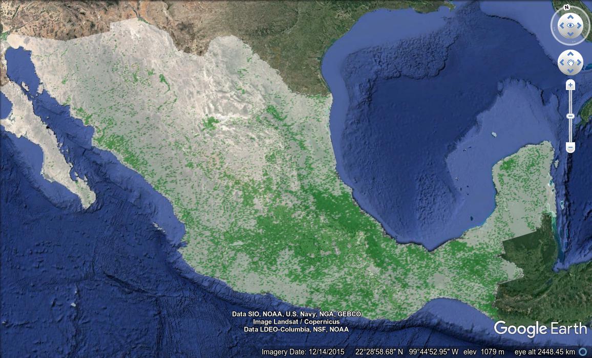
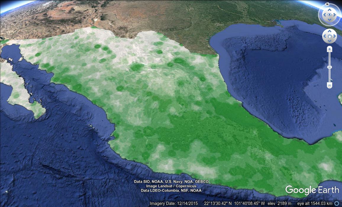
The resulting image, again with 500x500 pixel resolution, shows evidence of its circle-based counting heritage.

Obviously at this point, a person could mess with any number of variables to get all sorts of results. But for me it was enough to embed this as a GroundOverlay object within a simple KML file, to see the result in Google Earth:

postgres gis sql database