Our Blog

Systematic Query Building with Common Table Expressions

By Josh Tolley
June 12, 2018

The first time I got paid for doing PostgreSQL work on the side, I spent most of the proceeds on the mortgage (boring, I know), but I did get myself one little treat: a boxed set of DVDs from a favorite old television show. They became part of my evening ritual, watching an episode while cleaning the kitchen before bed. The show features three military draftees, one of whom, Frank, is universally disliked. In one episode, we learn that Frank has been unexpectedly transferred away, leaving his two roommates the unenviable responsibility of collecting Frank’s belongings and sending them to his new assignment. After some grumbling, they settle into the job, and one of them picks a pair of shorts off the clothesline, saying, “One pair of shorts, perfect condition: mine,” and he throws the shorts onto his own bed. Picking up another pair, he says, “One pair of shorts. Holes, buttons missing: Frank’s.”

The other starts on the socks: “One pair of socks, perfect condition: mine. One pair socks, holes: Frank’s. You know, this is going to be a lot easier than I thought.”

“A matter of having a system,” responds the first.

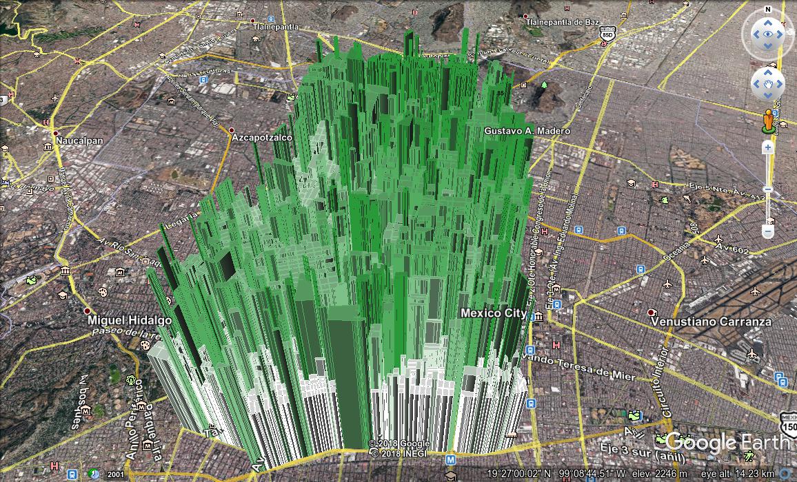
I find most things go better when I have a system, as a recent query writing task made clear. It involved data from the Instituto Nacional de Estadística y Geografía, or INEGI, an organization of the Mexican government tasked with collecting and managing country-wide statistics and geographical information. The data set contained the geographic outline of each city block in Mexico City, along with demographic and statistical data for each block: total population, a numeric score representing average educational level, how much of the block had sidewalks and landscaping, whether the homes had access to the municipal sewer and water systems, etc. We wanted to display the data on a Liquid Galaxy in some meaningful way, so I loaded it all in a PostGIS database and built a simple visualization showing each city block as a polygon extruded from the earth, with the height and color of the polygon proportional to the educational score for that block, compared to the city-wide average.

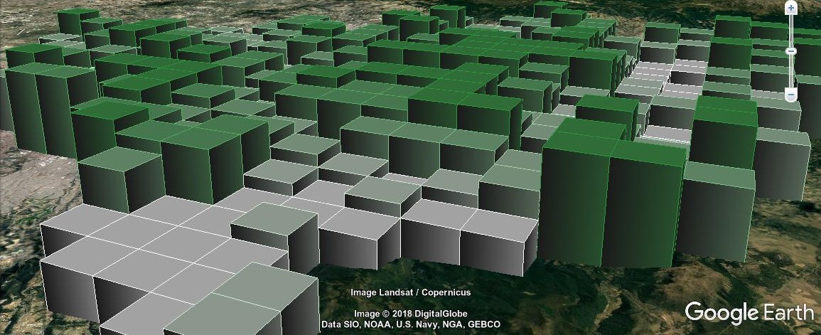
It wasn’t entirely a surprise that with so many polygons, rendering performance suffered a bit, but most of all the display was just plain confusing. This image is just one of Mexico City’s 16 boroughs.

With so much going on in the image, it’s difficult for the user to extract any meaningful information. So I turned to a technique we’d used in the past: reprocess the geographical area into grid squares, extrapolate the statistic of interest over the area of the square, and plot it again as a set of squares. The result is essentially a three dimensional heat map, much easier to comprehend, and, incidentally, to render.

As with most programming tasks, it’s helpful to have a system, so I started by sketching out how exactly to produce the desired result. I planned to overlay the features in the data set with a grid, and then for each square in the grid, find all intersecting city blocks, a number representing the educational level of residents of that block, and what percentage of the block’s total area intersects each grid square. From that information I can extrapolate that block’s contribution to the grid square’s total educational score. The precise derivation of the score isn’t important for our purposes here; suffice it to say it’s a numeric value with no particular associated unit, whose value lies in its relation to the scores of other blocks. Residents of a block with a high score are, on average, probably more educated than residents of a lower-scoring block. For this query, a block with an average educational level of, say, 100 “points”, would contribute all 100 points to a grid square if the entire block lay within that square, 60 points if only 60% of it was within the square, and so on. In the end, I should be able to add up all the scores for each grid square, rank them against all other grid squares, and produce a visualization.

I suffer from the decidedly masochistic habit of doing whatever I can in a single query, while maintaining a desire for readable and maintainable code. Cramming everything into one query isn’t always a good technique, as I hope to illustrate in a future blog post, but it worked well enough in this instance, and provides a good example I wanted to share, of one way to use Common Table Expressions. They do for SQL what subroutines do for other languages, separating tasks into distinct units. A common table expression looks like this:

WITH alias AS (
    SELECT something FROM wherever
),
another_alias AS (
    SELECT another_thing FROM alias LEFT JOIN something_else
)
SELECT an, assortment, of, fields
FROM another_alias;

As shown by this example query, the WITH keyword precedes a list of named, parenthesized queries, each of which functions throughout the life of the query as though it were a full-fledged table. These pseudo-tables are called Common Table Expressions, and they allow me to make one table for each distinct function in what will prove to be a fairly complicated query.

Let’s go through the elements of our new query piece by piece. First, I want to store the results of the query, so I can create different visualizations without recalculating everything. So I’ll make this query create a new table filled with its results. In this case, I called the table grid_mza_vals.

Now, for my first CTE. This query involves a few user-selected parameters, and I want an easy way to adjust these settings as I experiment to get the best results. I’ll want to fiddle with the number of grid squares in the overall result, as well as the coefficients used later on to calculate the height of each polygon. So my first CTE is called simply params, and returns a single row, composed of these parameters.

CREATE TABLE grid_mza_vals AS
WITH params AS (
    SELECT
        25 AS numsq,
        3800 AS alt_bias,
        500 AS alt_percfactor
),

The numsq value represents the number of grid squares along one edge of my overall grid; we’ll discuss the other values later. I’ve chosen a relatively small number of total grid squares for faster processing while building the rest of the query. I can make it more detailed, if I want, after everything else works.

The next thing I want is a sequence of numbers from 1 to numsq:

range AS (
    SELECT GENERATE_SERIES(0, numsq - 1) AS rng
    FROM params
),

Now I can join the range CTE with itself, to get the coordinates for each grid square:

gridix AS (
    SELECT
        x.rng AS x_ix,
        y.rng AS y_ix
    FROM range x, range y
),

Occasionally I like to check my progress, running whatever bits of the query I’ve already written to review its behavior. CTEs make this convenient, because I can adjust the final clause of the query to select data from whichever of the CTEs I’m currently interested in. Here’s the query thus far:

inegi=# WITH params AS (
    SELECT
        25 AS numsq,
        3800 AS alt_bias,
        500 AS alt_percfactor
),
range AS (
    SELECT GENERATE_SERIES(0, numsq - 1) AS rng
    FROM params
),
gridix AS (
    SELECT
        x.rng AS x_ix,
        y.rng AS y_ix
    FROM range x, range y
)
SELECT * FROM gridix;

 x_ix | y_ix
------+------
    0 |    0
    0 |    1
    0 |    2
    0 |    3
    0 |    4
    0 |    5
    0 |    6
    0 |    7
    0 |    8
    0 |    9
    0 |   10
    0 |   11
    0 |   12
    0 |   13
...

So far, so good. The gridix CTE returns coordinates for each cell in the grid, from zero to the numsq value from my params CTE. From those coordinates, if I know the geographic boundaries of the data set and the number of squares in each edge, I can calculate the latitude and longitude of the four corners of each grid square. First, I need to find the geographic boundaries of the data. My dataset lives in a table called manzanas, Spanish for “city block” (and also “apple”). Each row contains one geographic attribute containing a polygon defining the boundaries of the block, and several other attributes such as the education score I mentioned. In PostGIS there are several different ways to find the bounding box I want; here’s the one I used.

limits AS (
    SELECT
        MIN(ST_XMin(geom)) AS xmin,
        MAX(ST_XMax(geom)) AS xmax,
        MIN(ST_YMin(geom)) AS ymin,
        MAX(ST_YMax(geom)) AS ymax
    FROM
        manzanas
),

And, just to check my results:

inegi=#     SELECT
        MIN(ST_XMin(geom)) AS xmin,
        MAX(ST_XMax(geom)) AS xmax,
        MIN(ST_YMin(geom)) AS ymin,
        MAX(ST_YMax(geom)) AS ymax
    FROM
        manzanas;
     xmin      |     xmax     |       ymin       |       ymax
---------------+--------------+------------------+------------------
 -99.349658451 | -98.94668802 | 19.1241898199991 | 19.5863775499992
(1 row)

So the data in question extend from about 99.35 to 98.95 west longitude, and 19.12 to 19.59 north latitude. Now I’ll calculate the boundaries of each grid square, compose a text representation for the square in Well-Known Text format, and convert the text to a PostGIS geometry object. There’s another way I could do this, much simpler and probably much faster, which I hope to detail in a future blog post, but this will do for now.

gridcoords AS (
    SELECT
        (xmax - xmin) / numsq * x_ix + xmin AS x0,
        (xmax - xmin) / numsq * (x_ix + 1) + xmin AS x1,
        (ymax - ymin) / numsq * y_ix + ymin AS y0,
        (ymax - ymin) / numsq * (y_ix + 1) + ymin AS y1,
        x_ix || ',' || y_ix AS grid_ix
    FROM limits, params, gridix
),
gridewkt AS (
    SELECT
        grid_ix,
        'POLYGON((' ||
        x0 || ' ' || y0 || ',' ||
        x1 || ' ' || y0 || ',' ||
        x1 || ' ' || y1 || ',' ||
        x0 || ' ' || y1 || ',' ||
        x0 || ' ' || y0 || '))' AS ewkt
    FROM gridcoords
),
gridgeom AS (
    SELECT
        grid_ix, ewkt,
        ST_GeomFromText(ewkt, 4326) AS geom
    FROM gridewkt
),

And again, I’ll check the result by SELECTing grid_ix, ewkt, and geom, from the first row of the gridgeom CTE.

-[ RECORD 1 ]-----------------------------------------------------------------------------------------------------------------------------------------------------------------------------------------------
grid_ix | 0,0
ewkt    | POLYGON((-99.349658451 19.1241898199991,-99.34562874669 19.1241898199991,-99.34562874669 19.1288116972991,-99.349658451 19.1288116972991,-99.349658451 19.1241898199991))
geom    | 0103000020E6100000010000000500000029F4D6CD60D658C06B646FE7CA1F3340D3E508C81ED658C06B646FE7CA1F3340D3E508C81ED658C0EC3DABCDF920334029F4D6CD60D658C0EC3DABCDF920334029F4D6CD60D658C06B646FE7CA1F3340

I won’t claim an ability to translate the geometry object as represented above, but the ewkt value looks correct, so let’s keep going. Next I need to cut the blocks into pieces, corresponding to the parts of each block that belong in a single grid square. So a block lying entirely in one square will return one row in this next query; a block that intersects two squares will return two rows. Each row will include the geometries of the block, the square, and the intersection of the two, the total area of the block, the area of the intersection, and the total educational score for the block.

block_part AS (
    SELECT
        grid_ix,                     -- Grid square coordinates, e.g. 0,0
        m.gid AS manz_gid,           -- Manzana identifier
        ggm.geom,                    -- Grid square geometry
        m.graproes::FLOAT,           -- Educational score
        ST_Intersection(m.geom, ggm.geom)
            AS manz_bg_int,          -- Geometric intersection between grid square and city block
        ST_Area(m.geom)
            AS manz_area,            -- Area of the city block
        ST_Area(ST_Intersection(m.geom, ggm.geom)) / ST_Area(m.geom)
            AS manz_area_perc        -- Area of the intersection
    from
        gridgeom ggm
        JOIN manzanas m
            ON (ST_Intersects(m.geom, ggm.geom))
    WHERE
        m.graproes IS NOT NULL       -- Skip null educational scores
),

Here’s a sample of those results:

-[ RECORD 1 ]--+---------------------
grid_ix        | 15,16
manz_gid       | 61853
geom           | 0103000020E610000...
graproes       | 11
manz_bg_int    | 0103000020E610000...
manz_area      | 3.26175061395103e-06
manz_area_perc | 0.149256808754461
-[ RECORD 2 ]--+---------------------
grid_ix        | 15,17
manz_gid       | 61853
geom           | 0103000020E610000...
graproes       | 11
manz_bg_int    | 0103000020E610000...
manz_area      | 3.26175061395103e-06
manz_area_perc | 0.850743191246843

These results, which I admit to having selected with some care, show a single block, number 61853, which lies across the border between two grid squares. Now we’ll calculate the education score for each block fragment, and then divide the fragments into groups based on the grid square in which they belong, and aggregate the results. I did this in two separate CTEs.

grid_calc AS (
    SELECT
        grid_ix,
        geom,
        graproes * manz_area_perc AS grid_graproes,
        manz_area_perc
    FROM
        block_part
),
grid_accum AS (
    SELECT
        grid_ix,
        geom,
        SUM(grid_graproes) AS sum_graproes
    FROM grid_calc
    GROUP BY grid_ix, geom
),

This latest CTE gives results such as these:

-[ RECORD 1 ]+-----------------
grid_ix      | 12,14
geom         | 0103000020E61...
sum_graproes | 3888.53630440106

Now we’re left with turning these results into a visualization. I’d like to assign each polygon a height, and a color. To make the visualization easier to understand, I’ll divide the results into a handful of classes, and assign a height and color to each class.

Using an online color palette generator, I came up with a sequence of six colors, which progress from white to a green similar to the green bar on the Mexican flag. Another CTE will return these colors as an array, and yet another will assign the grid squares to groups based on their calculated score. Finally, a third will select the proper color from the array using that group value. At this point, readers are probably thinking “enough already; quit dividing everything into ever smaller CTEs”, to which I can only say, “Yeah, you may be right.”

colors AS (
    SELECT ARRAY['ffffff','d4ead7','a9d6af','7ec188','53ad60','299939'] AS colors
),
colorix AS (
    SELECT *,
        NTILE(ARRAY_LENGTH(colors, 1)) OVER (ORDER BY sum_graproes asc) AS edu_colorix
    FROM grid_accum, colors
),
color AS (
    SELECT *,
        colors[edu_colorix] as edu_color
    from colorix
)

The ntile() window function is useful for this kind of thing. It divides the given partition into buckets, and returns the number of the bucket for each row. Here, the partition consists of the whole data set; we sort it by educational score to ensure low-scoring grid squares get low-numbered buckets. Note also that I can change the colors, adding or removing groups, simply by adjusting the colors CTE. This could theoretically prove handy, if I decided I didn’t like the number of levels or the color scheme, but it’s a feature I never used for this visualization.

We’re on the home stretch, at last, and I should clarify how I plan to turn the database objects into KML, usable on a Liquid Galaxy. I used ogr2ogr from the GDAL toolkit. It converts between a number of different GIS data sources, including PostGIS to KML. I need to feed it the geometry I want to draw, as well as styling instructions and, in this case, a custom KML altitudeMode.

Styling is an involved topic; for our purposes it’s enough to say that I’ll tell ogr2ogr to use our selected color both to draw the lines of our polygons, and to fill them in. But moving the grid square’s geometry to an altitude corresponding to its educational score is fairly easy, using PostGIS’s ST_Force3DZ() function to add to the hitherto two-dimensional polygon a zero-valued third dimension, and ST_Translate() to move it above the surface of the earth a ways. So I can probably finish this with one final query:

-- Insert all previous CTEs here
SELECT
    ST_Translate(
        ST_Force3DZ(geom), 0, 0,
        alt_bias + edu_colorix * alt_percfactor
    ) AS edu_geom,
    'BRUSH(fc:#' || edu_color || 'ff);PEN(c:#' || edu_color || 'ff)' AS edu_style,
    'absolute' AS "altitudeMode"
FROM color, params;

You may remember alt_bias and alt_percfactor, the oddly named and thus far unexplained values in my first params CTE. These I used to control how far apart in altitude one group of polygons is from another, and to bias them all far enough above the ground to avoid the problem of them being obscured by terrain features. You may also remember that this query began with the CREATE TABLE grid_mza_vals AS... command, meaning that we’ll store the results of all this processing in a table, so ogr2ogr can get to it. We call ogr2ogr like this:

ogr2ogr \
    -f LIBKML education.kml \
    PG:"dbname=inegi user=josh password=<redacted>" \
    -sql "SELECT grid_ix, edu_geom, edu_style as \"OGR_STYLE\", \"altitudeMode\" FROM grid_mza_vals"

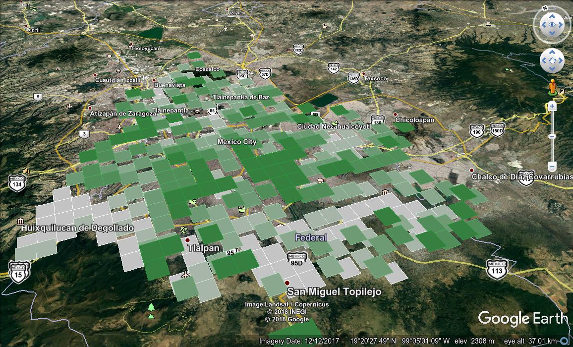
OGR’s LIBKML driver knows an attribute called “OGR_STYLE” is a style string, and one called “altitudeMode” is, predictably, the feature’s altitude mode. So this will create a KML file, containing one placemark for each row in our grid_mza_tables table. Each placemark consists of a colored square, floating in the air above Mexico City. The squares come in six different levels and six different colors, corresponding to our original education data. Something like this:

Here’s one of the placemarks from the KML.

      <Placemark id="sql_statement.1">
        <Style>
          <LineStyle>
            <color>ffffffff</color>
            <width>1</width>
          </LineStyle>
          <PolyStyle>
            <color>ffffffff</color>
          </PolyStyle>
        </Style>
        <ExtendedData>
          <SchemaData schemaUrl="#sql_statement.schema">
            <SimpleData name="grid_ix">11,10</SimpleData>
            <SimpleData name="OGR_STYLE">BRUSH(fc:#ffffffff);PEN(c:#ffffffff)</SimpleData>
          </SchemaData>
        </ExtendedData>
        <Polygon>
          <altitudeMode>absolute</altitudeMode>
          <outerBoundaryIs>
            <LinearRing>
              <coordinates>
                -99.17235146136,19.3090649119991,4300
                -99.15623264412,19.3090649119991,4300
                -99.15623264412,19.3275524211991,4300
                -99.17235146136,19.3275524211991,4300
                -99.17235146136,19.3090649119991,4300
              </coordinates>
            </LinearRing>
          </outerBoundaryIs>
        </Polygon>
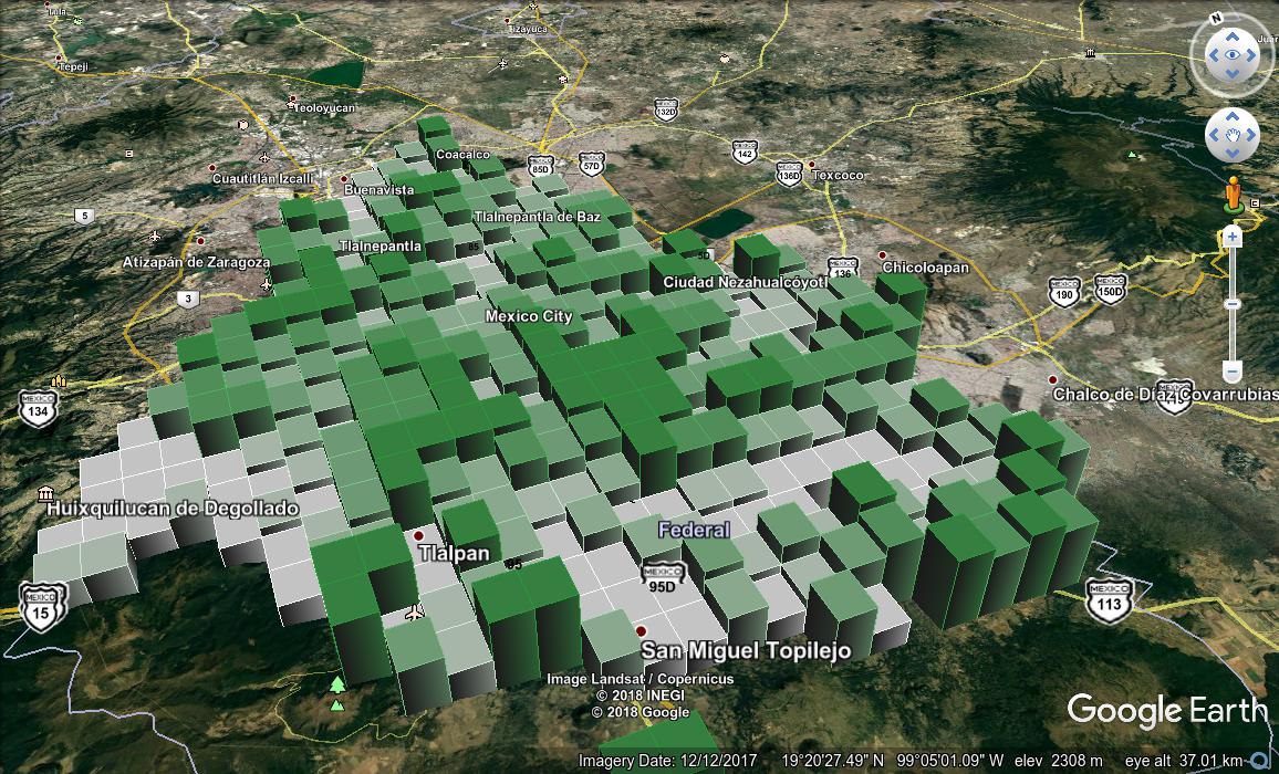
      </Placemark>

This may be sufficient, but it gets confusing when viewed from a low angle, because it’s hard to tell which square belongs to which part of the map. I prefer having the polygons “extruded” from the ground, as KML terms it. I used a simple Perl script to add the extrude element to each polygon in the KML, resulting in this:

This query works, but leaves a few things to be desired. For instance, doing everything in one query is probably not the best option when lots of processing is involved. Ideally we would calculate the grid geometries once, and save them in a table somewhere, for quicker processing as we build the rest of the query and experiment with visulization options. Second, PostGIS provides an arguably more elegant way of finding grid squares in the first place, a method which also affords other options for interesting visualizations. Stay tuned for a future blog post discussing these issues. Meanwhile, CTEs proved a valuable way to systematize and modularize a very complicated query.

postgres gis sql database