Our Blog

A/B Testing

By Kürşat Kutlu Aydemir
November 28, 2022

Photo by Mikhail Nilov

In statistics, A/B testing is “an experiment with two groups to establish which of two treatments, products, procedures, or the like is superior. Often one of the two treatments is the standard existing treatment, or no treatment” (Bruce 2020, 88).

A/B testing is very useful when adapted to e-commerce and marketing for determining the better of two options for a webpage.

Let’s consider a website where we want to analyze the page visits of page A and page B. Page A is the existing page (the control group), and page B is a new design of the web page (the treatment group).

To prepare A/B testing we start with the following steps:

1. Define hypotheses: null hypothesis (H₀) and alternative hypothesis.
2. Prepare control and treatment groups.

Then we’ll apply the A/B test on the dataset.

Purpose

The new and existing versions of our web page can show different performance in terms of marketing, visitor attention, and “conversion” to a particular goal. By applying A/B tests we can understand which of the two web pages has better performance. We can also find out if any difference in performance is due to chance or due to a design change.

Example

For example, let’s say we want to compare the conversion rates for visitors of page A and page B. Here are the aggregated results of our collected data for both pages:

Page A

Conversions: 231
Non-conversion visits: 11779

Page B

Conversions: 196
Non-conversion visits: 9823

The data to be sampled can vary. A very simple dataset could be a list of numeric results of observations: spent time on a control and a treatment web page, the weight of patients with and without treatments, etc. The permutation sampling of these results would be simply picking the values from the combined list of both groups.

In our conversion example the nature of the groups is similar but the values are slightly different, as they store two states: conversion and not conversion. However, we can still use a simple statistic like the mean to make our permutation test calculation.

Null hypothesis

Let’s build our null hypothesis around our experiment. In this example the null hypothesis would be “conversion rate of A ≥ conversion rate of B”. So, the alternative hypothesis would be “conversion rate of B > conversion rate of A”.

In a significance test we usually aim to answer the question of whether we will reject the null hypothesis or fail to reject the null hypothesis.

Data preprocessing and clean-up

Since the conversion/not conversion results are just yes/no (binary) results we might prefer to store them as values of 1 or 0.

We will use Python with the pandas library to import conversion samples for Pages A and B as a pandas Series:

import pandas as pd
import random

conversion = [1] * 427
conversion.extend([0] * 21602)
random.shuffle(conversion)
conversion = pd.Series(conversion)

Permutation test

To determine if the difference between the control and treatment groups is due to chance or not we can use permutation testing.

Permutation sampling is performed using the following steps, as listed in Practical Statistics (see the Reference section at the end):

1. Combine the results from the different groups into a single data set.
2. Shuffle the combined data and then randomly draw (without replacement) a resample of the same size as group A (which will contain some data from multiple groups).
3. From the remaining data, randomly draw (without replacement) a resample of the same size as group B.
4. Do the same for groups C, D, and so on. You have now collected one set of resamples that mirror the sizes of the original samples.
5. Whatever statistic or estimate was calculated for the original samples (in our case, the percent difference between two groups), calculate it now for the resamples, and record. This constitutes one permutation iteration.
6. Repeat the previous steps R times to yield a permutation distribution of the test statistic.

For each step of the permutation test we need to calculate the percent difference between successful and unsuccessful conversions. Using our example aggregated data from above, we can do this like so:

observed_percentage_diff = 100 * (196 / (196 + 9823) - 231 / (231 + 11779))

Which results in 0.032885893156042734 for our observation.

Below is a simple permutation test implementation from Practical Statistics.

def perm_fun(x, nA, nB):
    n = nA + nB
    idx_B = set(random.sample(range(n), nB))
    idx_A = set(range(n)) - idx_B
    return x.loc[list(idx_B)].mean() - x.loc[list(idx_A)].mean()

Now we need to repeat the sampling with a high R value, we’ll use 5000.

R = 5000
perm_diffs = [100 * perm_fun(conversion, 12010, 10019) for _ in range(R)]

Results

perm_diffs holds the percentage differences of the sampling data we generated. Now we have permutation test sampling differences and observed difference to be plotted.

import matplotlib.pyplot as plt

plt.hist(perm_diffs, bins=15)
plt.axvline(x = observed_percentage_diff, color='black', lw=2)
plt.show()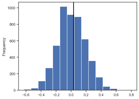

This plot shows us that the observed difference is well within the confidence level. Although we can easily identify the location observation, it is always good to check the p-value to be sure.

In this example our p-value is found with:

import numpy as np

p_value = np.mean([diff > observed_percentage_diff for diff in perm_diffs])

This results in 0.4204 for our data. Then we compare p_value with an alpha value, which is usually 0.05. If the p-value is less then alpha then we reject the null hypothesis. So in our example the p-value is extremely high, meaning we fail to reject the null hypothesis. Therefore, we can say that the difference between group A and group B is most likely due to chance rather than the treatment we applied.

Conclusion

The results of a significance test do not explicitly accept the null hypothesis, but rather help to understand if the treatments are affecting the results of the experiments or the results are most likely due to chance. A/B (or in some cases more groups, like C/D/E…) experiments are helpful to understand whether the treatment or chance is most likely the cause of the results, as well as finding which group performs the best.

Reference

Bruce, Peter, Andrew Bruce, and Peter Gedeck. Practical Statistics for Data Scientists, 2nd Edition. O’Reilly Media, Inc., 2020.

testing data-science