Understanding Linear Regression

By Kürşat Kutlu Aydemir
June 1, 2022

Linear regression is a regression model which outputs a numeric value. It is used to predict an outcome based on a linear set of input.
The simplest hypothesis function of linear regression model is a univariate function as shown in the equation below:
$$ h_θ = θ_0 + θ_1x_1 $$
As you can guess this function represents a linear line in the coordinate system. The hypothesis function (h0) approximates the output given input.
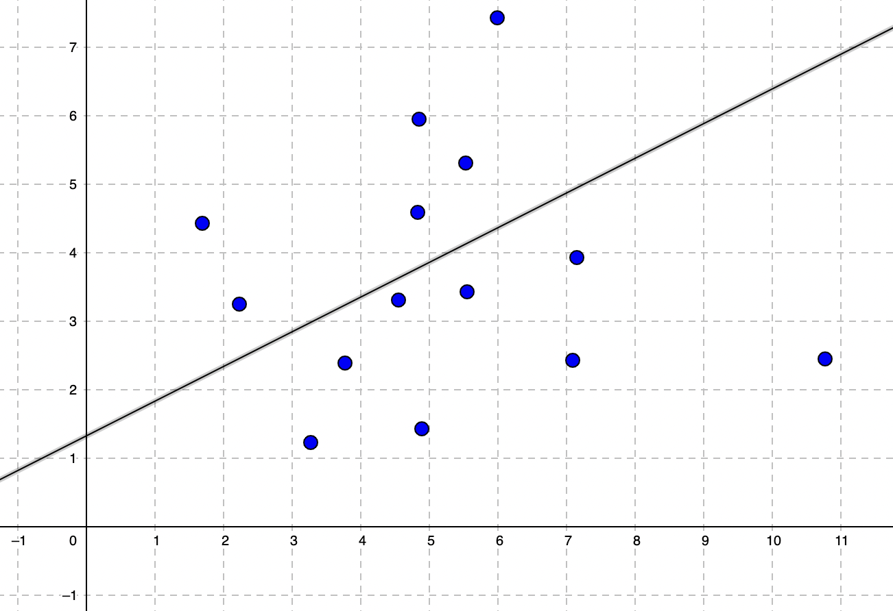
θ0 is the intercept, also called bias term. θ1 is the gradient or slope.
A linear regression model can either represent a univariate or a multivariate problem. So we can generalize the equation of the hypothesis as summation:
$$ h_θ = \sum{θ_ix_i} $$
where x0 is always 1.
We can also represent the hypothesis equation with vector notation:
$$ h_θ = \begin{bmatrix} θ_0 & θ_1 & θ_2 \dots θ_n \end{bmatrix} x \begin{bmatrix} x_0 \\ x_1 \\ x_2 \\ \vdots \\ x_n \end{bmatrix} $$
Linear Regression Model
I am going to introduce a linear regression model using a gradient descent algorithm. Each iteration of a gradient descent algorithm calculates the following steps:
- Hypothesis h
- The loss
- Gradient descent update
The gradient descent update iteration stops when it reaches the convergence.
Although I am implementing a univariate linear regression model in this section, these steps apply to multivariate linear regression models as well.
Hypothesis
We start the initial hypothesis assumption with random parameters. Then we calculate the loss using L2 Loss function over the training dataset. In Python:
def hypothesis(X, theta):
    return theta[0] + theta[1:] * X
In this function we took X input (univariate in this implementation) and theta parameter values. X represents the feature input of our dataset. Theta is the weights of the features. θ0 is called the bias term and θ1 is the gradient or slope.
L2 Loss Function
L2 Loss function — sometimes called Mean Squared Error (MSE) — is the total error of the current hypothesis over the given training dataset. During the training, by calculating the MSE, we can target minimizing the cumulative error.
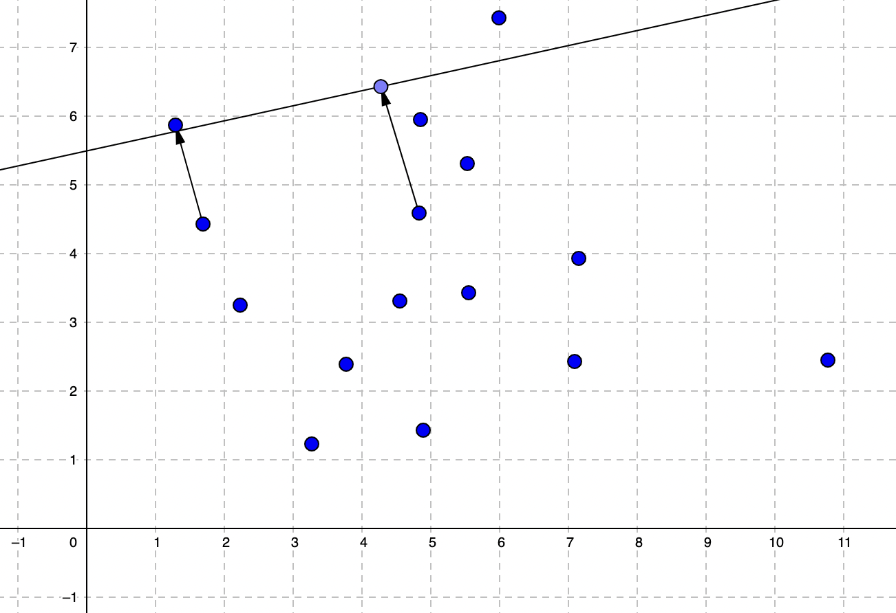
$$ J(θ) = \frac{\sum{(h_θ(x_i) - y_i)^2}}{2m} $$
L2 loss function (MSE) simply calculates the error by summing the squares of each data point error by dividing the size of the dataset.
The more the linear function is aligned, the optimized center of the data points with an optimized slope would give us a minimized error which is our target in linear regression training.
Gradients of the Loss
Each time we iterate and calculate a new theta (θ), we get a new theta1 (slope) value. If we plot each slope value in the gradient descent batch update we will have a curve like this:
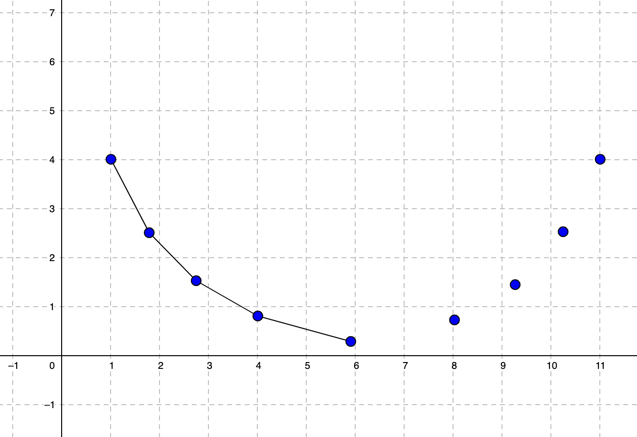
This curve has a minimum value which can’t get lower. Our goal is to find an optimal low value of theta1 that reaches a point where our curve doesn’t get lower anymore or the change can be ignored. That is where the convergence is achieved and the loss is minimized.
Let’s do a little bit more math. The gradient of the loss is the partial derivative of θ. We calculate partial differential of loss for θ0 and θ1 separately. For multivariate functions our θ1 is a generalized version for all available θi since the partial derivatives are calculated similarly. You can simply calculate the partial derivatives of loss function yourself too.
$$ \frac{∂}{∂θ_0}J(θ_0) = \frac{\sum{(h_0 - y_0)}}{m} $$
$$ \frac{∂}{∂θ_0}J(θ_i) = \frac{\sum{(h_i - y_i)x_i}}{m} $$
Since we know the hypothesis equation we can replace it in the derivatives as well:
def partial_derivatives(h, X, y):
    return [np.mean((h.flatten() - y)), np.mean((h.flatten() - y) * X.flatten())]
Now we will calculate the gradients for given hypothesis given theta, X, and y:
def calc_gradients(theta, X, y):
    gradient = [0, 0]

    h = hypothesis(X, theta)
    gradient = partial_derivatives(h, X, y)
    return np.array(gradient)
Batch Gradient Descent
The gradient descent method I used in this implementation is called batch gradient descent which uses all the data available through the iterations, which slows down the overall convergence process. There are methods to improve the performance of gradient descent such as stochastic gradient descent.
Since we calculated the gradients for the given theta we will iterate as much as we can until the convergence.
$$ θ_1(new) = θ_1(current) - α * J’(θ_1(current)) $$
Here comes the convergence rate or so called learning rate (α) factor to decide how long we should jump through the iterations. If α is too small, convergence can be more accurate, but the performance will be too small. This also leads to overfitting. If α is too big, the performance will be better, but convergence couldn’t be calculated accurately or well enough.
There is no strict best value for α since it depends on the dataset for training the model. By evaluating the model you trained you can find the best alpha value for your dataset. You can refer to statistical measures like R2 score to determine the observed variance. But there usually won’t be single model parameter, hyperparameter, or statistical variable to refer to for regularization.
def gradient_update(X, y, theta, alpha, stop_threshold):
    # initial loss
    loss = L2_loss(hypothesis(X, theta), y)
    old_loss = loss + stop_threshold

    while( abs(old_loss - loss) > stop_threshold ):
        # gradient descent update
        gradients = calc_gradients(theta, X, y)
        theta = theta - alpha * gradients
        old_loss = loss
        loss = L2_loss(hypothesis(X, theta), y)

    print('Gradient Descent training stopped at loss %s, with coefficients: %s' % (loss, theta))
    return theta
By performing batch gradient descent we actually train our algorithm and make it find the best theta values to fit the linear function. Now we can evaluate our algorithm and compare it with Sci-Kit Learn Linear Regression.
Evaluation
Since linear regression is a regression model, you should train and evaluate this model on regression datasets.
SK-Learn Diabetes dataset is a good regression dataset example. Below I loaded and prepared the dataset by splitting into training and test datasets.
from sklearn import datasets
from sklearn.model_selection import train_test_split

# Load the diabetes dataset
diabetes = datasets.load_diabetes()
diabetes_X = diabetes.data[:, np.newaxis, 2]
diabetes_y = diabetes.target

X_train, X_test, y_train, y_test = train_test_split(diabetes.data, diabetes_y, test_size=0.1)
Now we can evaluate our model:
from sklearn.metrics import mean_squared_error, r2_score

# initial random theta
theta = [100, 3]

stop_threshold = 0.1

# learning rate
alpha = 0.5

theta = gradient_update(X_train, y_train, theta, alpha, stop_threshold)
y_pred = hypothesis(X_test, theta)

print("Intercept (theta 0):", theta[0])
print("Coefficients (theta 1):", theta[1])
print("MSE:", mean_squared_error(y_test, y_pred))
print("R2 Score", r2_score(y_test, y_pred))

# Plot outputs using test data
plt.scatter(X_test, y_test,  color='black')
plt.plot(X_test, y_pred, color='blue', linewidth=3)

plt.show()
When I run my linear regression model it finds the optimal theta values, finishes the training, and outputs as below. I noted sample evaluation scores below too.
Gradient Descent training stopped at loss 3753.11429796413, with coefficients: [151.6166715  850.81024746]
Intercept (theta 0): 151.61667150054697
Coefficients (theta 1): 850.8102474614635
MSE: 5320.89741757879
R2 Score 0.14348916154815183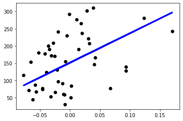
Now let’s evaluate the SK-Learn linear regression model with the same training and test datasets we used. I’m going to use default parameters without optimizing.
# Sci-Kit Learn LinearRegression model evaluation

regr = linear_model.LinearRegression()
regr.fit(X_train, y_train)
y_pred = regr.predict(X_test)

print("Coef:", regr.coef_)
print("Intercept:", regr.intercept_)
print("MSE:", mean_squared_error(y_test, y_pred))
print("R2 Score", r2_score(y_test, y_pred))

# Plot outputs
plt.scatter(X_test, y_test, color='black')
plt.plot(X_test, y_pred, color='blue', linewidth=3)

plt.show()
The output and plot of the SK-Learn Linear Regression model is as below:
Coef: [993.14228074]
Intercept: 151.5751918329106
MSE: 5544.283378702411
R2 Score 0.10753047228113943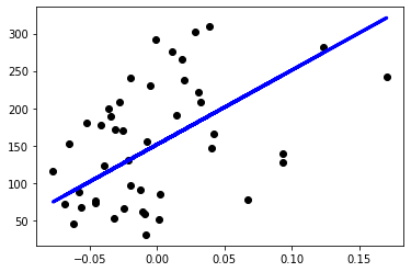
Notice the intercept of my linear regression model and SK-Learn’s linear regression model are very close with value of around ~151. MSE values are calculated very close too. Also both plotted their predictions very similarly as well.
Multivariate Linear Regression
We can add more features as we have more features in a dataset and prepare our hypothesis as below, similar to a univariate hypothesis.
$$ h_θ(x) = θ_0 + θ_1x_1 + … + θ_nx_n $$
A multivariate dataset can have multiple features and a single output like below.
| Feature1 | Feature2 | Feature3 | Feature4 | Target |
|---|---|---|---|---|
| 2 | 0 | 0 | 100 | 12 |
| 16 | 10 | 1000 | 121 | 18 |
| 5 | 5 | 450 | 302 | 14 |
Each feature is an independent variable (xi) of a dataset. Parameters (theta) are what we aim to find during the training just like the univariate model.
Linear Regression with Polynomial Functions
Sometimes a line function doesn’t fit the data well enough. Although if we are dealing with a polynomial function (having multiple features with exponential versions), it could fit the data better.
In this case the data itself is not linear but we are lucky that the parameter space is linear and we can still apply the linear regression over the non-linear dataset as well:
$$ h_θ(x) = θ_0 + θ_1x + θ_1x^2 … + θ_nx^n $$
$$ h_θ = \begin{bmatrix} 1 & x & x^2 \dots x^n \end{bmatrix} x \begin{bmatrix} θ_0 \\ θ_1 \\ θ_2 \\ \vdots \\ θ_n \end{bmatrix} $$
Here the data is non-linear but the parameters are linear and we can still apply the gradient descent algorithm.
Conclusion
In this post I implemented a linear regression model from scratch and evaluated by training it.
Linear regression is useful when your dataset variables can be related in a linear relation. In the real world, linear regression is very useful in forecasting.
machine-learning data-science python
Comments