Speech Recognition from scratch using Dilated Convolutions and CTC in TensorFlow

By Kamil Ciemniewski
January 8, 2019
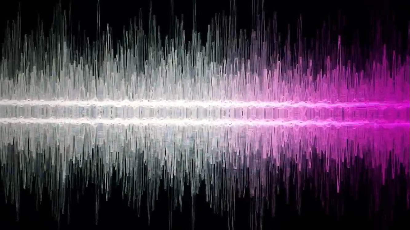
Image by WILL POWER · CC BY 2.0, cropped
In this blog post, I’d like to take you on a journey. We’re going to get a speech recognition project from its architecting phase, through coding and training. In the end, we’ll have a fully working model. You’ll be able to take it and run the model serving app, exposing a nice HTTP API. Yes, you’ll even be able to use it in your projects.
Speech recognition has been amongst one of the hardest tasks in Machine Learning. Traditional approaches involve meticulous crafting and extracting of the audio features that separate one phoneme from another. To be able to do that, one needs a deep background in data science and signal processing. The complexity of the training process prompted teams of researchers to look for alternative, more automated approaches.
With the growing development of Deep Learning, the need for handcrafted features declined. The training process for a neural network is much more streamlined. You can feed the signals either in their raw form or as their spectrograms and watch the model improve.
Did this get you excited? Let’s start!
Project Plan of Attack
Let’s build a web service that exposes an API. Let it be able to receive audio signals, encoded as an array of floating point numbers. In return, we’re going to get the recognized text.
Here’s a rough plan of the stages we’re going to go through:
- Get the dataset to train the model on
- Architect the model
- Implement it along with the unit tests
- Train it on the dataset
- Measure its accuracy
- Serve it as a web service
The dataset
The open-source community has a lot to be thankful for the Mozilla Foundation for. It’s a host of many projects with a wonderful, free Firefox browser at its forefront. One of its other projects, called Common Voice, focuses on gathering large data sets to be used by anyone in speech recognition projects.
The datasets consist of wave files and their text transcriptions. There’s no notion of time-alignment. It’s just the audio and text for each utterance.
If you want to code along, head up to the Common Voice Datasets download page. Be warned that it weighs roughly around 12GB.
After the download, simply extract the files from the archive into the ./data directory of the root of the project. The files, in the end, should reside under the ./data/cv_corpus_v1/ path.
How much data should we have? It always depends on the challenge at hand. Roughly speaking, the more difficult the task, the more powerful your neural network needs to be. It will need to be capable of expressing more complex patterns in data. The more powerful the network, the easier it is to have it just memorize the training examples. This is highly undesirable and results in overfitting. To lessen its aptitude to do so, you need to either augment your data on the fly randomly or gather more “real” examples. On this project, we’re going to do both. Data augmentation will be covered in the coding section. Additional datasets we’ll use are well known LibriSpeech (the file to download, around 23GB) and VoxForge (the file to download).
Those two datasets are among the most popular that are freely available. There are others I chose to omit as they weigh quite a lot. I was already almost out of free space after the download and preprocessing of the three sets chosen above.
You need to download both Libri and Vox and extract them under ./data/LibriSpeech/ and ./data/voxforge/.
Background on audio processing
In order to build a working model, we need some background in signal processing. Although a lot of the traditional work is going to be done by the neural network automatically, we still need to understand what is going on in order to reason about its various hyperparameters.
Additionally, we’re going to process audio into a form that’s easier to train. This is going to lower the memory requirements. It’s also going to lower the time needed for model’s parameters to converge to ones that work well.
How is audio represented?
Let’s have a quick look at what the audio data looks like when we load it from a wave file.
import librosa
import librosa.display

SAMPLING_RATE=16000

# ...

wave, _ = librosa.load(path_to_file, sr=SAMPLING_RATE)

librosa.display.waveplot(wave, sr=SAMPLING_RATE)
The above code specifies that we want to load the audio data with a sampling rate of a 16k (more about it later). It then loads it and plots it along the time axis:

The X-axis obviously represents the time. The Y axis is often called the amplitude. A quick look at the plot above makes it obvious that we have negative values in the signal. How come those values are called amplitudes then? Amplitude is said to represent the maximum difference of displacements of a physical object as it vibrates. What does it mean to have a negative amplitude? To make those values a bit more clear, let’s call it just displacement for now. Audio is nothing else than the vibration of the air. If you were to build an electrical recorder, you might come up with one that gives you output in voltages at each point in time. As the air vibrates, you need a reference point obviously. This, in turn, allows you to catch the exact specifics of the vibration — how it “rises” above the reference point and then gets back way below it. Imagine that your electrical circuit gives you output within the range of -1V and 1V. To load it into your computer and into the plot like above, you’d need to capture those values at discrete points in time. The sampling rate is nothing else than a number of times within one second when the value from your sound-meter would be measured and stored — to be loaded later. Next time, when you read that your CD from the ’90 contains audio sampled at a frequency of 44,100 Hz, you’ll know that the raw “air displacement” values were sampled 44,100 times each second.
Let’s do a simple thought experiment to prepare for the next section. What would you hear if all the above values were constant, e.g. 1.0? We saw that the values given by librosa are floating points. In the example file they ranged between -0.6 and 0.6. The value of 1.0 is certainly much higher — would you hear “more” of “something” then? Because the definition of a sound is that it’s a vibration: you wouldn’t hear anything! The amplitudes of the audio signal must periodically change — this is how we detect or hear sounds. This implies that in order to distinguish between different sounds, those sounds have to “vibrate differently”. The difference that makes sounds different is the frequency of the vibration.
Decomposing the signal with the Fourier Transform
Let’s create a signal generating machine, that will output a sinusoidal of a given frequency and amplitude:
def gen_sin(freq, amplitude, sr=1000):
    return np.sin(
        (freq * 2 * np.pi * np.linspace(0, sr, sr)) / sr
    ) * amplitude
Here’s how 1000 points signal looks like for a frequency of 30 and an amplitude of 1:
import seaborn as sns

sns.lineplot(data=gen_sin(30, 1))
Here’s one for 10 and 0.6:

You can count the number of times the values in plots approach their maximum. Knowing that sine has only one maximum within its period and that we’re showing just one second, that number shows that we have frequencies 30 and 10.
What would we get if we were to sum such sinusoidal signals of different frequencies and amplitudes? Let’s see — below you can see 3 different sine waves plotted on top of each other. The fourth — and last one — shows the signal that is the sum of all of them:

Here’s another example, with the last plot showing the sum of 5 different waves:

It isn’t that regular anymore, is it? It turns out that you can construct any signal by summing up some number of sine waves of different frequencies and amplitudes (and phases, their translation in time). The converse is also true: any signal can be represented as a sum of some number of sine waves of different frequencies and amplitudes (and phases). This is extremely important to our speech recognition task. Frequencies are the real difference between sounds that make up the phonemes and words that we want to be able to recognize.
This is where the Fourier Transform comes into play. It takes our data points that represent intensity per each point in time and produces data points representing intensity per each frequency bin. It’s said that it transforms the domain of the signal from time into frequency. Now, what exactly is a frequency bin? Imagine the physical audio signal being constructed from frequencies between 0Hz and 8000Hz. The FFT algorithm (Fast Fourier Transform) is going to split that full spectrum into bins. If you were to split it into 10 bins, you’d end up having the following ranges: 0Hz–800Hz, 800Hz–1600Hz, 1600Hz–2400Hz, 2400Hz–3200Hz, 3200Hz–4000Hz, 4000Hz–4800Hz, 4800Hz–5600Hz, 5600Hz–6400Hz, 6400Hz–7200Hz, 7200Hz–8000Hz.
Let’s see how the FFT works on the example of the signal given above. The waves and plots were produced by the following Python function:
def plot_wave_composition(defs, hspace=1.0):
    fig_size = plt.rcParams["figure.figsize"]

    plt.rcParams["figure.figsize"] = [14.0, 10.0]

    waves = [
        gen_sin(freq, amp)
        for freq, amp in defs
    ]

    fig, axs = plt.subplots(nrows=len(defs) + 1)

    for ix, wave in enumerate(waves):
        sb.lineplot(data=wave, ax=axs[ix])
        axs[ix].set_ylabel('{}'.format(defs[ix]))

        if ix != 0:
            axs[ix].set_title('+')

    plt.subplots_adjust(hspace = hspace)

    sb.lineplot(data=sum(waves), ax=axs[len(defs)])
    axs[len(defs)].set_ylabel('sum')
    axs[len(defs)].set_xlabel('time')
    axs[len(defs)].set_title('=')

    plt.rcParams["figure.figsize"] = fig_size

    return waves, sum(waves)
We can plot the signals and grab them at the same time with:
wave_defs = [
        (2, 1),
        (3, 0.8),
        (5, 0.2),
        (7, 0.1),
        (9, 0.25)
    ]

waves, the_sum = plot_wave_composition(wave_defs)
Next, let’s compute the FFT values along with the frequencies:
ffts = np.fft.fft(the_sum)
freqs = np.fft.fftfreq(len(the_sum))

frequencies, coeffs = zip(
    *list(
        filter(
            lambda row: row[1] > 10, # arbitrary threshold but let’s not make it too complex for now
            [ (int(abs(freq * 1000)), coef) for freq, coef in zip(freqs[0:(len(ffts) // 2)], np.abs(ffts)[0:(len(ffts) // 2)]) ]
        )
    )
)

sns.barplot(x=list(frequencies), y=coeffs)
The last call produces the following plot:

The X-axis represents now the frequency in Hz, while the Y-axis is the intensity.
There’s one missing part before we can use it with our speech data. As you can see, FFT gives us frequencies for the whole signal, assuming that it’s periodic and spans in time into infinity. Obviously, when I say “hello”, the air vibrates differently in the beginning, changes in between and is even more different at the end. We need to split that audio into small “windows” of data points. By feeding them into FFT, we can get the frequencies for each one of them. This turns the data domain from time into frequency within the scope of the window. It remains the info about the time at the global level, making our data represent: time x frequency x intensity.
Scaling frequencies
The human perception is a vastly complex phenomenon. Taking that into account can take us a long way when working on the recognition model emulating the work of our brains when we’re listening to each other.
Let’s make another experiment. What sound is produced by the 800Hz sine?
from IPython.display import Audio

Audio(data=gen_sin(800, 1, 16000), rate=16000)
Let’s now generate 900Hz and 1000Hz to get a sense of the difference:
900Hz:
1000Hz:
Let us now ante up the frequencies and generate 7000Hz, 7100Hz and 7200Hz:
Can you hear the difference being smaller in the case of the last three? It’s a well-known phenomenon. We sense a greater difference in sounds for lower frequencies and as it increases that difference becomes less and less.
Because of this, three gentlemen—Stevens, Volkmann, and Newman—created a so-called Mel scale in 1937. You can think of it as a simple rescaling of the frequencies that roughly follows the relationship shown below:
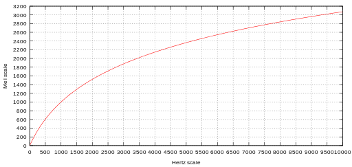
Although not mandatory, lots of models that deal with human speech also decrease the importance of the intensity by taking the log of the re-scaled data. The resulting time x frequency (mels) x log-intensity is called the log-Mel spectrogram.
Background on deep learning techniques in use for this project
We’ve just gone through the necessary basics of signal processing. Let’s now focus on the Deep Learning concepts we’ll use to construct and train the model.
While this article assumes that the reader already knows a lot, there are less common techniques we’ll use that deserve at least a quick go through.
Dilated convolutions as a faster alternative to recurrent networks
Traditionally, the sequence processing in Deep Learning is tackled by the recurrent neural networks.
No matter the choice of their flavor, the basic scheme is always the same: the computations are done sequentially going through examples in time. In our case, we’d need to split the time x frequency x intensity into time length of frequency x intensity chunks. As the chunks would be processed one by one, the recurrent network internal state would “remember” the previous chunk’s specifics, incorporating them into their future outputs. The output shape would be time x frequency x recurrent units.
The fact that the computations are done sequentially, makes them quite slow overall. Later in-pipeline computations spend most of the time waiting on the previous ones to finish because of the direct dependency. The problem is even more severe with the use of GPUs. We use them because of their ability to do math in parallel on huge chunks of data. With recurrent networks, lots of that power is being wasted.
The premise of RNNs is that in theory, they can have the capacity for keeping very long contexts in their “memory”. This has recently been put into test and falsified in practice by Bai et al. Also, when you stop and think about the task at hand: does it really matter to “remember” the beginning of the sentence to know that it ends with the word “dog”? Some context is obviously needed — but not as wide as it might seem at first.
I have an Nvidia GTX 1070Ti with 8GB of memory to train my models on. I don’t really feel like waiting a month for my recurrent network to converge. In this project, let’s use a very performant alternative — convolutional neural network.
Expanding the context of the convolutional network
Simple convolutional layers weren’t used for sequence processing much for a good reason. The crux of the sequence processing is to be able to take bigger contexts into account. Depending on the job, we might want to constrain the context only to the past — learning the causal relations in data. We might sometimes want to incorporate both past and future in it as well. The go-to solution for doing OCR at the moment is to use bidirectional recurrent layers. Their one pass learns the relations from left to right while another learns from right to left. The results are then concatenated.
By applying proper padding, we can easily include one or two-sided contexts in 1D convolutions. The challenge is that in order to make the outputs depend on bigger contexts, the size of the filters needs to become bigger and bigger. This, in turn, requires more and more memory.
Because our aim is to create a model that we’ll be able to train on a quite cheap (given the GPUs used in this field usually) GTX 1070Ti (around $500 at the moment), we want the memory requirements to be as low as possible.
Thanks to the success of the WaveNet (among others), a specific class of convolutional layers gained a lot of attention lately. The variation is called Dilated Convolutions or sometimes Atrous Convolutions. So what are they?
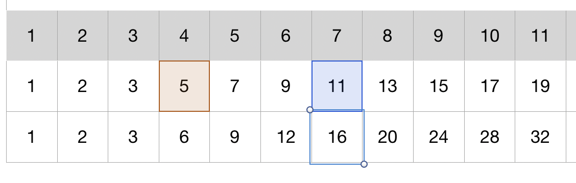
Let’s first have a look at how the outputs depend on their context for simple convolutional layers:
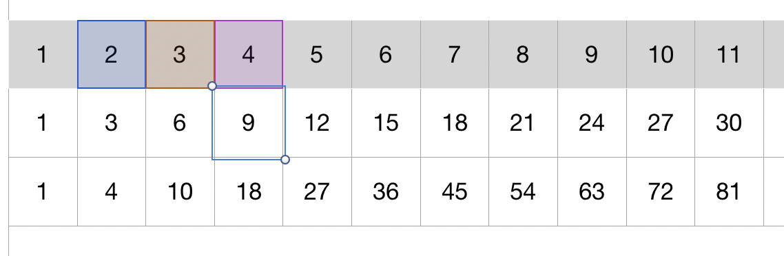
Imagine that you originally have just the top-most row of numbers. You are going to use 1D convolutions and to make the reasoning easiest, the number of filters is 1. Also for simplicity, all filter values are set to 1. You can see the cross-correlation (because that’s what convolutional layers are in fact computing) operator taking 3 values in the context, multiplying by the filter and summing up to 2 * 1 + 3 * 1 + 4 * 1 = 9.
The atrous convolutions are really the same, except they dilate their focus without increasing the size of the filter by introducing holes. It’s shown below with the convolution of the size 2 and dilation of 2:
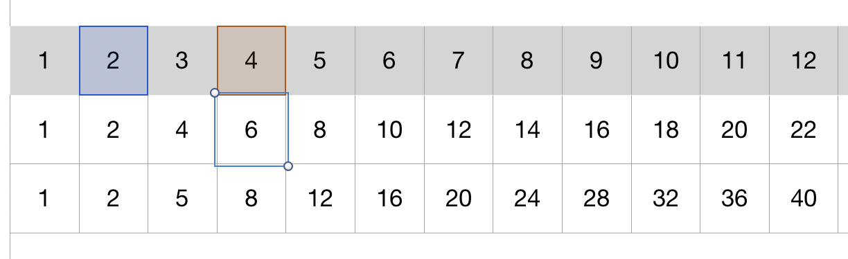
Here’s yet another example for the size of 2 and dilation of 3:
Gated activations
Traditionally, convolutional layers are followed by the *elu family of activations (ReLu, Elu, PRelu, Selu). They fit in well within the “match pattern” paradigm of the conv nets. On the contrary, recurrent units operate the “remember/forget” approach. Two of their most commonly used implementations, GRU and LSTM, include explicit “forget” gates.
We want to mimic their ability to “forget” parts of the context within our dilated convolutions based model too. To do that, we’re going to use the “gated activations” approach, explained by Liptchinsky et al.
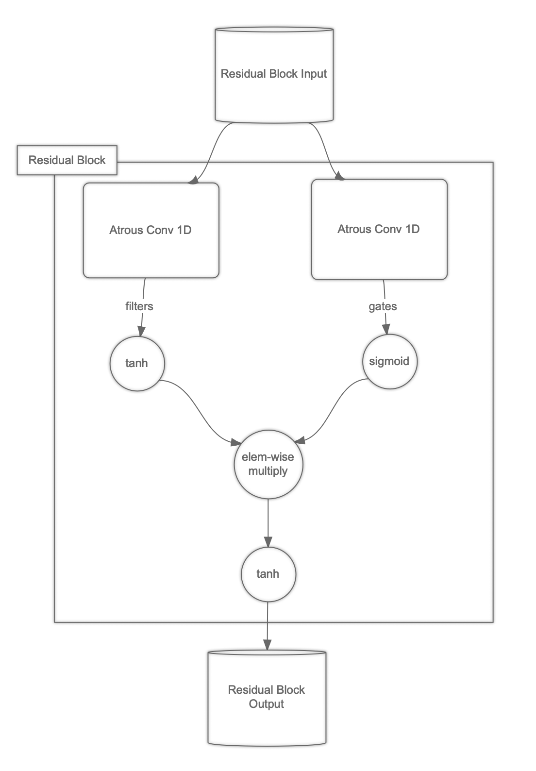
The idea is very simple: we pass the input through Conv1D separately and apply tanh and sigmoid respectively. The result is the element-wise product. We’re going to go one step further in our approach, by applying tanh one more time in the end.
Others
The full explanation of all of the details of our neural network’s architecture is beyond the scope of an article like this. Let me point you at additional pieces along with the reading they come from:
Let’s code it
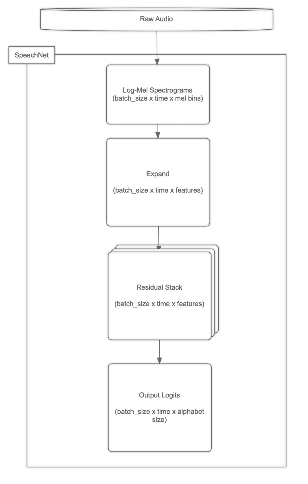
The architecture of our choice in this project is going to heavily rely on the great success of residual-style networks as well as dilated convolutions. You might see similarities to the famous WaveNet, although it’s going to be a bit different.
Here is the bird-eye view of the SpeechNet neural network:
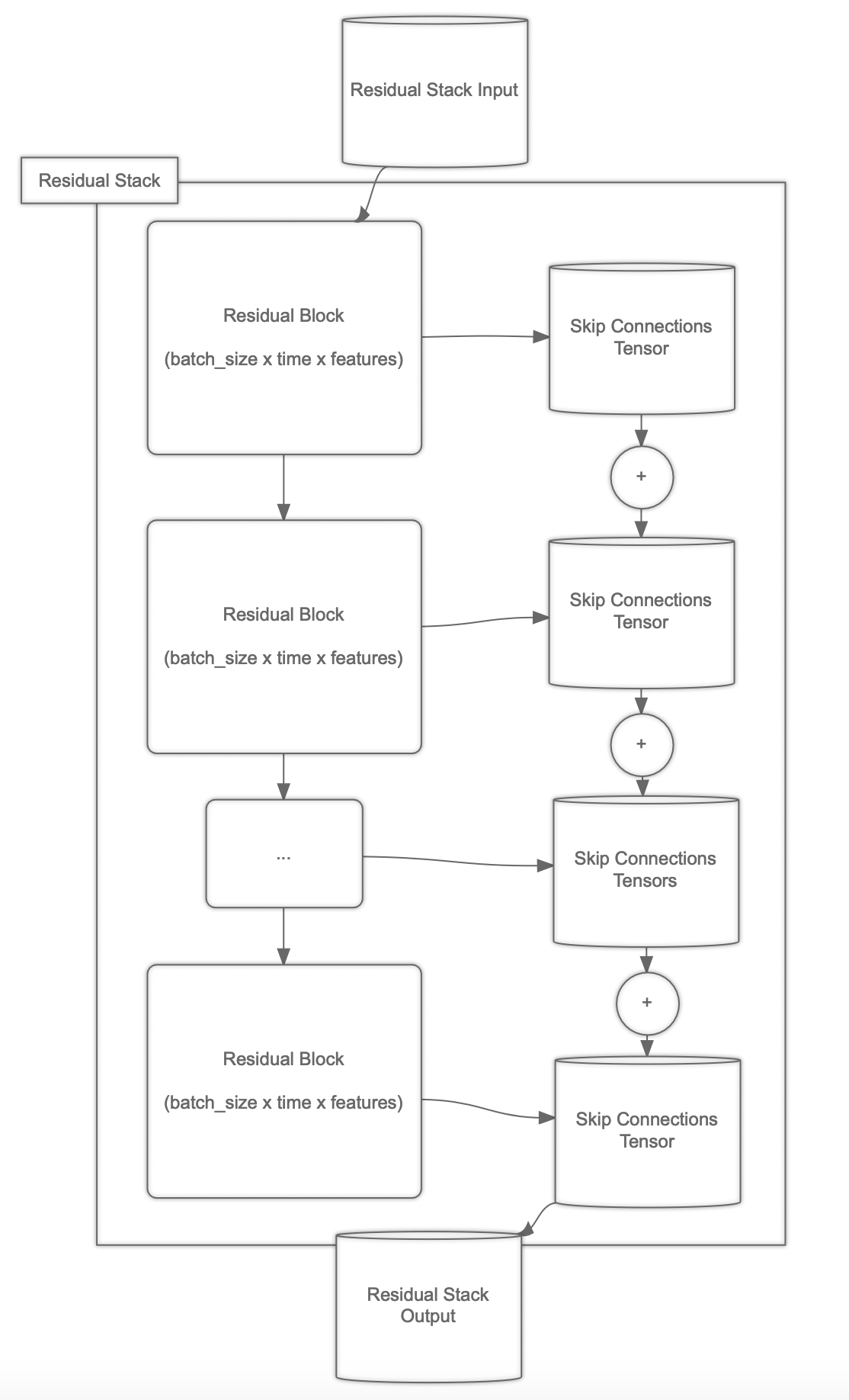
The residual stacks, being at the heart of it, are structured the following way:
The residual blocks, doing all the heavy lifting, can be seen as shown below:
The most important aspect of coding of the Deep Learning models
Developing Deep Learning models doesn’t really differ that much from any other type of coding. It does require specific background knowledge, but the good coding practices remain the same. In fact, good coding habits are 10× more relevant here than in e.g. a web-app project.
Training a speech-to-text model is bound to require days if not weeks. Imagine having a small bug in your code, preventing the process from finding a good local minimum. It’s extremely frustrating to find out about it days into the training, with the model trainable parameters not being improved much.
Let’s start by adding some unit tests then. In this project, we’re using the Jupyter notebook as we don’t intend to package it anywhere. The code’s intent is to be for educational purposes mainly.
Adding unit tests within the Jupyter notebook is possible with the following “hack” (notice the value for argv):
import unittest

RUN_TESTS = TRUE

class TestNotebook(unittest.TestCase):
    def test_it_works(self):
        self.assertEqual(2 + 2, 4)

if __name__ == '__main__' and RUN_TESTS:
    import doctest

    doctest.testmod()
    unittest.main(
        argv=['first-arg-is-ignored'],
        failfast=True,
        exit=False
    )
You can notice the import of the doctest module which adds support for doc-string level tests which may come in handy as well.
I also hugely recommend the hypothesis library for testing the QuickCheck way as I blogged about it before.
Data pipeline
A place that’s surprisingly very bug-potent is the data pipeline. It’s easy to e.g. shuffle the labels independently of input vectors if you’re not careful. There’s also always a chance to introduce input vectors including NaN or inf values, which a few steps later produce NaN or inf loss values. Let’s add a simple test to check for the first condition:
# assuming test path will look like: 1/file.wav
# the input and output types are driven by the input_fn shown later
# here, we’re just generating values based on the “path”
def dummy_load_wave(example):
    row, params = example
    path = row.filename

    return np.ones((SAMPLING_RATE)) * float(path.split('/')[0]), row

class TestNotebook(unittest.TestCase):

    # (...)

    def test_dataset_returns_data_in_order(self):

        params = experiment_params(
            dataset_params(
                batch_size=2,
                epochs=1,
                augment=False
            )
        )

        data = pd.DataFrame(
            data={
                'text': [ str(i) for i in range(10) ],
                'filename':  [ '{}/wav'.format(i) for i in range(10) ]
            }
        )

        dataset = input_fn(data, params['data'], dummy_load_wave)()
        iterator = dataset.make_one_shot_iterator()
        next_element = iterator.get_next()

        with tf.Session() as session:
            try:
                while True:
                    audio, label = session.run(next_element)
                    audio, length = audio

                    for _audio, _label in zip(list(audio), list(label)):
                        self.assertEqual(_audio[0], float(_label))

                    for _length in length:
                        self.assertEqual(_length, SAMPLING_RATE)
            except tf.errors.OutOfRangeError:
                pass
The above code assumes having the input_fn function in scope. If you’re not familiar with the concept yet, please go ahead and read the introduction to the TensorFlow Estimators API.
Here’s our implementation:
from multiprocessing import Pool

def input_fn(input_dataset, params, load_wave_fn=load_wave):
    def _input_fn():
        """
        Returns raw audio wave along with the label
        """

        dataset = input_dataset

        print(params)

        if 'max_text_length' in params and params['max_text_length'] is not None:
            print('Constraining dataset to the max_text_length')
            dataset = input_dataset[input_dataset.text.str.len() < params['max_text_length']]

        if 'min_text_length' in params and params['min_text_length'] is not None:
            print('Constraining dataset to the min_text_length')
            dataset = input_dataset[input_dataset.text.str.len() >= params['min_text_length']]

        if 'max_wave_length' in params and params['max_wave_length'] is not None:
            print('Constraining dataset to the max_wave_length')

        print('Resulting dataset length: {}'.format(len(dataset)))

        def generator_fn():
            pool = Pool()
            buffer = []

            for epoch in range(params['epochs']):
                for _, row in dataset.sample(frac=1).iterrows():
                    buffer.append((row, params))

                    if len(buffer) >= params['batch_size']:

                        if params['parallelize']:
                            audios = pool.map(
                                load_wave_fn,
                                buffer
                            )
                        else:
                            audios = map(
                                load_wave_fn,
                                buffer
                            )

                        for audio, row in audios:
                            if audio is not None:
                                if np.isnan(audio).any():
                                    print('SKIPPING! NaN coming from the pipeline!')
                                else:
                                    yield (audio, len(audio)), row.text.encode()

                        buffer = []

        return tf.data.Dataset.from_generator(
                generator_fn,
                output_types=((tf.float32, tf.int32), (tf.string)),
                output_shapes=((None,()), (()))
            ) \
            .padded_batch(
                batch_size=params['batch_size'],
                padded_shapes=(
                    (tf.TensorShape([None]), tf.TensorShape(())),
                    tf.TensorShape(())
                )
            )

    return _input_fn
This depends on the load_wave function:
import librosa
import hickle as hkl
import os.path

def to_path(filename):
    return './data/cv_corpus_v1/' + filename

def load_wave(example, absolute=False):
    row, params = example

    _path = row.filename if absolute else to_path(row.filename)

    if os.path.isfile(_path + '.wave.hkl'):
        wave = hkl.load(_path + '.wave.hkl').astype(np.float32)
    else:
        wave, _ = librosa.load(_path, sr=SAMPLING_RATE)
        hkl.dump(wave, _path + '.wave.hkl')

    if len(wave) <= params['max_wave_length']:
        if params['augment']:
            wave = random_noise(
                random_stretch(
                    random_shift(
                        wave,
                        params
                    ),
                    params
                ),
                params
            )
    else:
        wave = None

    return wave, row
Which depends on three other functions used to augment the data on the fly to improve the model’s generalization:
import random
import glob

noise_files = glob.glob('./data/*.wav')
noises = {}

def random_stretch(audio, params):
    rate = random.uniform(params['random_stretch_min'], params['random_stretch_max'])

    return librosa.effects.time_stretch(audio, rate)

def random_shift(audio, params):
    _shift = random.randrange(params['random_shift_min'], params['random_shift_max'])

    if _shift < 0:
        pad = (_shift * -1, 0)
    else:
        pad = (0, _shift)

    return np.pad(audio, pad, mode='constant')

def random_noise(audio, params):
    _factor = random.uniform(
        params['random_noise_factor_min'],
        params['random_noise_factor_max']
    )

    if params['random_noise'] > random.uniform(0, 1):
        _path = random.choice(noise_files)

        if _path in noises:
            wave = noises[_path]
        else:
            if os.path.isfile(_path + '.wave.hkl'):
                wave = hkl.load(_path + '.wave.hkl').astype(np.float32)
                noises[_path] = wave
            else:
                wave, _ = librosa.load(_path, sr=SAMPLING_RATE)
                hkl.dump(wave, _path + '.wave.hkl')
                noises[_path] = wave

        noise = random_shift(
            wave,
            {
                'random_shift_min': -16000,
                'random_shift_max': 16000
            }
        )

        max_noise = np.max(noise[0:len(audio)])
        max_wave = np.max(audio)

        noise = noise * (max_wave / max_noise)

        return _factor * noise[0:len(audio)] + (1.0 - _factor) * audio
    else:
        return audio
Notice that we’re making almost everything into a configurable parameter. We want the code to allow the greatest freedom of searching for just the right set of hyperparameters.
The data pipeline as shown above randomly shuffles the Pandas data frame once for each epoch. It also creates a pool of background workers to parallelize the data loading as much as possible. We’re doing the data loading and augmentation on the CPU. It also uses the hickle library for caching audio signals on the disk. Loading a wave file with a given sampling rate isn’t that fast as one might think. In my experiments, loading the resulting array of floating points via hickle was 10x faster. We need the best speed of feeding the data into the network or else our GPU is going to stay underutilized.
In my experiments also, turning data augmentation on made a real difference. I’ve run the training without it and the network overfit was disastrous: with the normalized edit distance for the training set revolving around 0.01 and 0.53 for the validation.
The random_noise function uses the noise sounds included in the Speech Commands: A public dataset for single-word speech recognition dataset. Please go ahead and download it, extracting just the noise files under the ./data directory.
The last function in use we haven’t seen yet is the experiment_params. It’s just a helper that allows an easy params hash construction for our experiments:
def dataset_params(batch_size=32,
                   epochs=50000,
                   parallelize=True,
                   max_text_length=None,
                   min_text_length=None,
                   max_wave_length=80000,
                   shuffle=True,
                   random_shift_min=-4000,
                   random_shift_max= 4000,
                   random_stretch_min=0.7,
                   random_stretch_max= 1.3,
                   random_noise=0.75,
                   random_noise_factor_min=0.2,
                   random_noise_factor_max=0.5,
                   augment=False):
    return {
        'parallelize': parallelize,
        'shuffle': shuffle,
        'max_text_length': max_text_length,
        'min_text_length': min_text_length,
        'max_wave_length': max_wave_length,
        'random_shift_min': random_shift_min,
        'random_shift_max': random_shift_max,
        'random_stretch_min': random_stretch_min,
        'random_stretch_max': random_stretch_max,
        'random_noise': random_noise,
        'random_noise_factor_min': random_noise_factor_min,
        'random_noise_factor_max': random_noise_factor_max,
        'epochs': epochs,
        'batch_size': batch_size,
        'augment': augment
    }
Labels encoder and decoder
When working with the CTC loss, we need a way to code each letter as a numerical value. Conversely, the neural network is going to give us probabilities for each letter, given by its index within the output matrix.
The idea behind this project’s approach is to push the encoding and decoding into the network graph itself. We want two functions: encode_labels and decode_codes. We want the first to turn a string into an array of integers. The second one should complement it, turning the array of integers into the resulting string.
It’s a good idea to use our hypothesis library for this unit test. It’s going to come up with many input examples, trying to falsify our assumptions:
@given(st.text(alphabet="abcdefghijk1234!@#$%^&*", max_size=10))
def test_encode_and_decode_work(self, text):
    assume(text != '')

    params = { 'alphabet': 'abcdefghijk1234!@#$%^&*' }

    label_ph = tf.placeholder(tf.string, shape=(1), name='text')
    codes_op = encode_labels(label_ph, params)
    decode_op = decode_codes(codes_op, params)

    with tf.Session() as session:
        session.run(tf.global_variables_initializer())
        session.run(tf.tables_initializer(name='init_all_tables'))

        codes, decoded = session.run(
            [codes_op, decode_op],
            {
                label_ph: np.array([text])
            }
        )

        note(codes)
        note(decoded)

        self.assertEqual(text, ''.join(map(lambda s: s.decode('UTF-8'), decoded.values)))
        self.assertEqual(codes.values.dtype, np.int32)
        self.assertEqual(len(codes.values), len(text))
Here is the implementation that passes the above test:
def encode_labels(labels, params):
    characters = list(params['alphabet'])

    table = tf.contrib.lookup.HashTable(
        tf.contrib.lookup.KeyValueTensorInitializer(
            characters,
            list(range(len(characters)))
        ),
        -1,
        name='char2id'
    )

    return table.lookup(
        tf.string_split(labels, delimiter='')
    )

def decode_codes(codes, params):
    characters = list(params['alphabet'])

    table = tf.contrib.lookup.HashTable(
        tf.contrib.lookup.KeyValueTensorInitializer(
            list(range(len(characters))),
            characters
        ),
        '',
        name='id2char'
    )

    return table.lookup(codes)
Log-Mel Spectrogram layer
Another piece we need is a way to turn raw audio signals into the log-Mel spectrograms. The idea, again, is to push it into the network graph. This way it’s going to work way faster on GPUs and also the model’s API is going to be much simpler.
In the following unit test, we’re testing our custom TensorFlow layer against values coming from known-to-be-valid librosa:
@given(
    st.sampled_from([22000, 16000, 8000]),
    st.sampled_from([1024, 512]),
    st.sampled_from([1024, 512]),
    npst.arrays(
        np.float32,
        (4, 16000),
        elements=st.floats(-1, 1)
    )
)
@settings(max_examples=10)
def test_log_mel_conversion_works(self, sampling_rate, n_fft, frame_step, audio):
    lower_edge_hertz=0.0
    upper_edge_hertz=sampling_rate / 2.0
    num_mel_bins=64

    def librosa_melspectrogram(audio_item):
        spectrogram = np.abs(
            librosa.core.stft(
                audio_item,
                n_fft=n_fft,
                hop_length=frame_step,
                center=False
            )
        )**2

        return np.log(
            librosa.feature.melspectrogram(
                S=spectrogram,
                sr=sampling_rate,
                n_mels=num_mel_bins,
                fmin=lower_edge_hertz,
                fmax=upper_edge_hertz,
            ) + 1e-6
        )

    audio_ph = tf.placeholder(tf.float32, (4, 16000))

    librosa_log_mels = np.transpose(
        np.stack([
            librosa_melspectrogram(audio_item)
            for audio_item in audio
        ]),
        (0, 2, 1)
    )

    log_mel_op = tf.check_numerics(
        LogMelSpectrogram(
            sampling_rate=sampling_rate,
            n_fft=n_fft,
            frame_step=frame_step,
            lower_edge_hertz=lower_edge_hertz,
            upper_edge_hertz=upper_edge_hertz,
            num_mel_bins=num_mel_bins
        )(audio_ph),
        message="log mels"
    )

    with tf.Session() as session:
        session.run(tf.global_variables_initializer())

        log_mels = session.run(
            log_mel_op,
            {
               audio_ph: audio
            }
        )

        np.testing.assert_allclose(
            log_mels,
            librosa_log_mels,
            rtol=1e-1,
            atol=0
        )
The implementation of the layer, that passes the above unit test reads as follows:
class LogMelSpectrogram(tf.layers.Layer):
    def __init__(self,
                 sampling_rate,
                 n_fft,
                 frame_step,
                 lower_edge_hertz,
                 upper_edge_hertz,
                 num_mel_bins,
                 **kwargs):
        super(LogMelSpectrogram, self).__init__(**kwargs)

        self.sampling_rate = sampling_rate
        self.n_fft = n_fft
        self.frame_step = frame_step
        self.lower_edge_hertz = lower_edge_hertz
        self.upper_edge_hertz = upper_edge_hertz
        self.num_mel_bins = num_mel_bins

    def call(self, inputs, training=True):
        stfts = tf.contrib.signal.stft(
            inputs,
            frame_length=self.n_fft,
            frame_step=self.frame_step,
            fft_length=self.n_fft,
            pad_end=False
        )

        power_spectrograms = tf.real(stfts * tf.conj(stfts))

        num_spectrogram_bins = power_spectrograms.shape[-1].value

        linear_to_mel_weight_matrix = tf.constant(
            np.transpose(
                librosa.filters.mel(
                    sr=self.sampling_rate,
                    n_fft=self.n_fft + 1,
                    n_mels=self.num_mel_bins,
                    fmin=self.lower_edge_hertz,
                    fmax=self.upper_edge_hertz
                )
            ),
            dtype=tf.float32
        )

        mel_spectrograms = tf.tensordot(
            power_spectrograms,
            linear_to_mel_weight_matrix,
            1
        )

        mel_spectrograms.set_shape(
            power_spectrograms.shape[:-1].concatenate(
                linear_to_mel_weight_matrix.shape[-1:]
            )
        )

        return tf.log(mel_spectrograms + 1e-6)
Converted data lengths function
In order to use the CTC loss and decoder efficiently, we need to pass it the length of the data effectively representing audio for each batch. This is because not all audio files are of the same length but we need to pad them with zeros to do mini-batch.
Here’s the unit test:
@given(
        npst.arrays(
            np.float32,
            (st.integers(min_value=16000, max_value=16000*5)),
            elements=st.floats(-1, 1)
        ),
        st.sampled_from([22000, 16000, 8000]),
        st.sampled_from([1024, 512, 640]),
        st.sampled_from([1024, 512, 160]),
    )
    @settings(max_examples=10)
    def test_compute_lengths_works(self,
                                   audio_wave,
                                   sampling_rate,
                                   n_fft,
                                   frame_step
                                  ):
        assume(n_fft >= frame_step)

        original_wave_length = audio_wave.shape[0]

        audio_waves_ph = tf.placeholder(tf.float32, (None, None), name="audio_waves")
        original_lengths_ph = tf.placeholder(tf.int32, (None), name="original_lengths")

        lengths_op = compute_lengths(
            original_lengths_ph,
            {
                'frame_step': frame_step,
                'n_fft': n_fft
            }
        )

        self.assertEqual(lengths_op.dtype, tf.int32)

        log_mel_op = LogMelSpectrogram(
            sampling_rate=sampling_rate,
            n_fft=n_fft,
            frame_step=frame_step,
            lower_edge_hertz=0.0,
            upper_edge_hertz=8000.0,
            num_mel_bins=13
        )(audio_waves_ph)

        with tf.Session() as session:
            session.run(tf.global_variables_initializer())

            lengths, log_mels = session.run(
                [lengths_op, log_mel_op],
                {
                    audio_waves_ph: np.array([audio_wave]),
                    original_lengths_ph: np.array([original_wave_length])
                }
            )

            note(original_wave_length)
            note(lengths)
            note(log_mels.shape)

            self.assertEqual(lengths[0], log_mels.shape[1])
And here’s the implementation:
def compute_lengths(original_lengths, params):
    """
    Computes the length of data for CTC
    """

    return tf.cast(
        tf.floor(
            (tf.cast(original_lengths, dtype=tf.float32) - params['n_fft']) /
                params['frame_step']
        ) + 1,
        tf.int32
    )
Atrous 1D Convolutions layer
It’s also a good idea to ensure that our dilated convolutions layer behaves as in theory. TensorFlow already includes an ability to specify the dilations. The end result though may differ wildly based on the choice of other parameters.
Let’s ensure at least that it works as intended when we choose it to work in the “causal” mode. The unit test:
def test_causal_conv1d_works(self):
    conv_size2_dilation_1 = AtrousConv1D(
        filters=1,
        kernel_size=2,
        dilation_rate=1,
        kernel_initializer=tf.ones_initializer(),
        use_bias=False
    )

    conv_size3_dilation_1 = AtrousConv1D(
        filters=1,
        kernel_size=3,
        dilation_rate=1,
        kernel_initializer=tf.ones_initializer(),
        use_bias=False
    )

    conv_size2_dilation_2 = AtrousConv1D(
        filters=1,
        kernel_size=2,
        dilation_rate=2,
        kernel_initializer=tf.ones_initializer(),
        use_bias=False
    )

    conv_size2_dilation_3 = AtrousConv1D(
        filters=1,
        kernel_size=2,
        dilation_rate=3,
        kernel_initializer=tf.ones_initializer(),
        use_bias=False
    )

    data = np.array(list(range(1, 31)))
    data_ph = tf.placeholder(tf.float32, (1, 30, 1))

    size2_dilation_1_1 = conv_size2_dilation_1(data_ph)
    size2_dilation_1_2 = conv_size2_dilation_1(size2_dilation_1_1)

    size3_dilation_1_1 = conv_size3_dilation_1(data_ph)
    size3_dilation_1_2 = conv_size3_dilation_1(size3_dilation_1_1)

    size2_dilation_2_1 = conv_size2_dilation_2(data_ph)
    size2_dilation_2_2 = conv_size2_dilation_2(size2_dilation_2_1)

    size2_dilation_3_1 = conv_size2_dilation_3(data_ph)
    size2_dilation_3_2 = conv_size2_dilation_3(size2_dilation_3_1)

    with tf.Session() as session:
        session.run(tf.global_variables_initializer())

        outputs = session.run(
            [
                size2_dilation_1_1,
                size2_dilation_1_2,
                size3_dilation_1_1,
                size3_dilation_1_2,
                size2_dilation_2_1,
                size2_dilation_2_2,
                size2_dilation_3_1,
                size2_dilation_3_2
            ],
            {
                data_ph: np.reshape(data, (1, 30, 1))
            }
        )

        for ix, out in enumerate(outputs):
            out = np.squeeze(out)
            outputs[ix] = out

            self.assertEqual(out.shape[0], len(data))

        np.testing.assert_equal(
            outputs[0],
            np.array([1, 3, 5, 7, 9, 11, 13, 15, 17, 19, 21, 23, 25, 27, 29, 31, 33, 35, 37, 39, 41, 43, 45, 47, 49, 51, 53, 55, 57, 59], dtype=np.float32)
        )

        np.testing.assert_equal(
            outputs[1],
            np.array([1, 4, 8, 12, 16, 20, 24, 28, 32, 36, 40, 44, 48, 52, 56, 60, 64, 68, 72, 76, 80, 84, 88, 92, 96, 100, 104, 108, 112, 116], dtype=np.float32)
        )

        np.testing.assert_equal(
            outputs[2],
            np.array([1, 3, 6, 9, 12, 15, 18, 21, 24, 27, 30, 33, 36, 39, 42, 45, 48, 51, 54, 57, 60, 63, 66, 69, 72, 75, 78, 81, 84, 87], dtype=np.float32)
        )

        np.testing.assert_equal(
            outputs[3],
            np.array([1, 4, 10, 18, 27, 36, 45, 54, 63, 72, 81, 90, 99, 108, 117, 126, 135, 144, 153, 162, 171, 180, 189, 198, 207, 216, 225, 234, 243, 252], dtype=np.float32)
        )

        np.testing.assert_equal(
            outputs[4],
            np.array([1, 2, 4, 6, 8, 10, 12, 14, 16, 18, 20, 22, 24, 26, 28, 30, 32, 34, 36, 38, 40, 42, 44, 46, 48, 50, 52, 54, 56, 58], dtype=np.float32)
        )

        np.testing.assert_equal(
            outputs[5],
            np.array([1, 2, 5, 8, 12, 16, 20, 24, 28, 32, 36, 40, 44, 48, 52, 56, 60, 64, 68, 72, 76, 80, 84, 88, 92, 96, 100, 104, 108, 112], dtype=np.float32)
        )

        np.testing.assert_equal(
            outputs[6],
            np.array([1, 2, 3, 5, 7, 9, 11, 13, 15, 17, 19, 21, 23, 25, 27, 29, 31, 33, 35, 37, 39, 41, 43, 45, 47, 49, 51, 53, 55, 57], dtype=np.float32)
        )

        np.testing.assert_equal(
            outputs[7],
            np.array([1, 2, 3, 6, 9, 12, 16, 20, 24, 28, 32, 36, 40, 44, 48, 52, 56, 60, 64, 68, 72, 76, 80, 84, 88, 92, 96, 100, 104, 108], dtype=np.float32)
        )
And the layer’s code:
class AtrousConv1D(tf.layers.Layer):
    def __init__(self,
                 filters,
                 kernel_size,
                 dilation_rate,
                 use_bias=True,
                 kernel_initializer=tf.glorot_normal_initializer(),
                 causal=True
                ):
        super(AtrousConv1D, self).__init__()

        self.filters = filters
        self.kernel_size = kernel_size
        self.dilation_rate = dilation_rate
        self.causal = causal

        self.conv1d = tf.layers.Conv1D(
            filters=filters,
            kernel_size=kernel_size,
            dilation_rate=dilation_rate,
            padding='valid' if causal else 'same',
            use_bias=use_bias,
            kernel_initializer=kernel_initializer
        )

    def call(self, inputs):
        if self.causal:
            padding = (self.kernel_size - 1) * self.dilation_rate
            inputs = tf.pad(inputs, tf.constant([(0, 0,), (1, 0), (0, 0)]) * padding)

        return self.conv1d(inputs)
Residual Block layer
One aspect that wasn’t covered yet is the heavy usage of batch normalization. When coding the residual block layer, ensuring that batch normalization is properly applied when training and when inferring is one of the most important tasks.
Here’s the unit test:
@given(
    npst.arrays(
        np.float32,
        (4, 16000),
        elements=st.floats(-1, 1)
    ),
    st.sampled_from([64, 32]),
    st.sampled_from([7, 3]),
    st.sampled_from([1, 4]),
)
@settings(max_examples=10)
def test_residual_block_works(self, audio_waves, filters, size, dilation_rate):
    with tf.Graph().as_default() as g:
        audio_ph = tf.placeholder(tf.float32, (4, None))

        log_mel_op = LogMelSpectrogram(
            sampling_rate=16000,
            n_fft=512,
            frame_step=256,
            lower_edge_hertz=0,
            upper_edge_hertz=8000,
            num_mel_bins=10
        )(audio_ph)

        expanded_op = tf.layers.Dense(filters)(log_mel_op)

        _, block_op = ResidualBlock(
            filters=filters,
            kernel_size=size,
            causal=True,
            dilation_rate=dilation_rate
        )(expanded_op, training=True)

        # really dumb loss function just for the sake
        # of testing:
        loss_op = tf.reduce_sum(block_op)

        variables = tf.trainable_variables()
        self.assertTrue(any(["batch_normalization" in var.name for var in variables]))

        grads_op = tf.gradients(
            loss_op,
            variables
        )

        for grad, var in zip(grads_op, variables):
            if grad is None:
                note(var)

            self.assertTrue(grad is not None)

        with tf.Session(graph=g) as session:
            session.run(tf.global_variables_initializer())

            result, expanded, grads, _ = session.run(
                [block_op, expanded_op, grads_op, loss_op],
                {
                    audio_ph: audio_waves
                }
            )

            self.assertFalse(np.array_equal(result, expanded))
            self.assertEqual(result.shape, expanded.shape)
            self.assertEqual(len(grads), len(variables))
            self.assertFalse(any([np.isnan(grad).any() for grad in grads]))
And here’s the implementation:
class ResidualBlock(tf.layers.Layer):
    def __init__(self, filters, kernel_size, dilation_rate, causal, **kwargs):
        super(ResidualBlock, self).__init__(**kwargs)

        self.dilated_conv1 = AtrousConv1D(
            filters=filters,
            kernel_size=kernel_size,
            dilation_rate=dilation_rate,
            causal=causal
        )

        self.dilated_conv2 = AtrousConv1D(
            filters=filters,
            kernel_size=kernel_size,
            dilation_rate=dilation_rate,
            causal=causal
        )

        self.out = tf.layers.Conv1D(
            filters=filters,
            kernel_size=1
        )

    def call(self, inputs, training=True):
        data = tf.layers.batch_normalization(
            inputs,
            training=training
        )

        filters = self.dilated_conv1(data)
        gates = self.dilated_conv2(data)

        filters = tf.nn.tanh(filters)
        gates = tf.nn.sigmoid(gates)

        out = tf.nn.tanh(
            self.out(
                filters * gates
            )
        )

        return out + inputs, out
Residual Stack layer
Testing the residual stack follows the same kind of logic:
@given(
    npst.arrays(
        np.float32,
        (4, 16000),
        elements=st.floats(-1, 1)
    ),
    st.sampled_from([64, 32]),
    st.sampled_from([7, 3])
)
@settings(max_examples=10)
def test_residual_stack_works(self, audio_waves, filters, size):
    dilation_rates = [1,2,4]

    with tf.Graph().as_default() as g:
        audio_ph = tf.placeholder(tf.float32, (4, None))

        log_mel_op = LogMelSpectrogram(
            sampling_rate=16000,
            n_fft=512,
            frame_step=256,
            lower_edge_hertz=0,
            upper_edge_hertz=8000,
            num_mel_bins=10
        )(audio_ph)

        expanded_op = tf.layers.Dense(filters)(log_mel_op)

        stack_op = ResidualStack(
            filters=filters,
            kernel_size=size,
            causal=True,
            dilation_rates=dilation_rates
        )(expanded_op, training=True)

        # really dumb loss function just for the sake
        # of testing:
        loss_op = tf.reduce_sum(stack_op)

        variables = tf.trainable_variables()
        self.assertTrue(any(["batch_normalization" in var.name for var in variables]))

        grads_op = tf.gradients(
            loss_op,
            variables
        )

        for grad, var in zip(grads_op, variables):
            if grad is None:
                note(var)

            self.assertTrue(grad is not None)

        with tf.Session(graph=g) as session:
            session.run(tf.global_variables_initializer())

            result, expanded, grads, _ = session.run(
                [stack_op, expanded_op, grads_op, loss_op],
                {
                    audio_ph: audio_waves
                }
            )

            self.assertFalse(np.array_equal(result, expanded))
            self.assertEqual(result.shape, expanded.shape)
            self.assertEqual(len(grads), len(variables))
            self.assertFalse(any([np.isnan(grad).any() for grad in grads]))
With the layer’s code looking as follows:
class ResidualStack(tf.layers.Layer):
    def __init__(self, filters, kernel_size, dilation_rates, causal, **kwargs):
        super(ResidualStack, self).__init__(**kwargs)

        self.blocks = [
            ResidualBlock(
                filters=filters,
                kernel_size=kernel_size,
                dilation_rate=dilation_rate,
                causal=causal
            )
            for dilation_rate in dilation_rates
        ]

    def call(self, inputs, training=True):
        data = inputs
        skip = 0

        for block in self.blocks:
            data, current_skip = block(data, training=training)
            skip += current_skip

        return skip
The SpeechNet
Finally, let’s add a very similar test for the SpeechNet itself:
@given(
    npst.arrays(
        np.float32,
        (4, 16000),
        elements=st.floats(-1, 1)
    )
)
@settings(max_examples=10)
def test_speech_net_works(self, audio_waves):
    with tf.Graph().as_default() as g:
        audio_ph = tf.placeholder(tf.float32, (4, None))

        logits_op = SpeechNet(
            experiment_params(
                {},
                stack_dilation_rates= [1, 2, 4],
                stack_kernel_size= 3,
                stack_filters= 32,
                alphabet= 'abcd'
            )
        )(audio_ph)

        # really dumb loss function just for the sake
        # of testing:
        loss_op = tf.reduce_sum(logits_op)

        variables = tf.trainable_variables()
        self.assertTrue(any(["batch_normalization" in var.name for var in variables]))

        grads_op = tf.gradients(
            loss_op,
            variables
        )

        for grad, var in zip(grads_op, variables):
            if grad is None:
                note(var)

            self.assertTrue(grad is not None)

        with tf.Session(graph=g) as session:
            session.run(tf.global_variables_initializer())

            result, grads, _ = session.run(
                [logits_op, grads_op, loss_op],
                {
                    audio_ph: audio_waves
                }
            )

            self.assertEqual(result.shape[2], 5)
            self.assertEqual(len(grads), len(variables))
            self.assertFalse(any([np.isnan(grad).any() for grad in grads]))
And let’s provide the code that passes it:
class SpeechNet(tf.layers.Layer):
    def __init__(self, params, **kwargs):
        super(SpeechNet, self).__init__(**kwargs)

        self.to_log_mel = LogMelSpectrogram(
            sampling_rate=params['sampling_rate'],
            n_fft=params['n_fft'],
            frame_step=params['frame_step'],
            lower_edge_hertz=params['lower_edge_hertz'],
            upper_edge_hertz=params['upper_edge_hertz'],
            num_mel_bins=params['num_mel_bins']
        )

        self.expand = tf.layers.Conv1D(
            filters=params['stack_filters'],
            kernel_size=1,
            padding='same'
        )

        self.stacks = [
            ResidualStack(
                filters=params['stack_filters'],
                kernel_size=params['stack_kernel_size'],
                dilation_rates=params['stack_dilation_rates'],
                causal=params['causal_convolutions']
            )
            for _ in range(params['stacks'])
        ]

        self.out = tf.layers.Conv1D(
            filters=len(params['alphabet']) + 1,
            kernel_size=1,
            padding='same'
        )

    def call(self, inputs, training=True):
        data = self.to_log_mel(inputs)

        data = tf.layers.batch_normalization(
            data,
            training=training
        )

        if len(data.shape) == 2:
            data = tf.expand_dims(data, 0)

        data = self.expand(data)

        for stack in self.stacks:
            data = stack(data, training=training)

        data = tf.layers.batch_normalization(
            data,
            training=training
        )

        return self.out(data) + 1e-8
The model function
We have only one last piece of code to cover before we’ll be able to start the training. It’s the model_fn that adheres to the TensorFlow Estimators API:
def model_fn(features, labels, mode, params):
    if isinstance(features, dict):
        audio = features['audio']
        original_lengths = features['length']
    else:
        audio, original_lengths = features

    lengths = compute_lengths(original_lengths, params)

    if labels is not None:
        codes = encode_labels(labels, params)

    network = SpeechNet(params)

    is_training = mode==tf.estimator.ModeKeys.TRAIN

    logits = network(audio, training=is_training)
    text, predicted_codes = decode_logits(logits, lengths, params)

    if mode == tf.estimator.ModeKeys.PREDICT:
        predictions = {
            'logits': logits,
            'text': tf.sparse_tensor_to_dense(
                text,
                ''
            )
        }

        export_outputs = {
            'predictions': tf.estimator.export.PredictOutput(predictions)
        }

        return tf.estimator.EstimatorSpec(
            mode,
            predictions=predictions,
            export_outputs=export_outputs
        )
    else:
        loss = tf.reduce_mean(
            tf.nn.ctc_loss(
                labels=codes,
                inputs=logits,
                sequence_length=lengths,
                time_major=False,
                ignore_longer_outputs_than_inputs=True
            )
        )

        mean_edit_distance = tf.reduce_mean(
            tf.edit_distance(
                tf.cast(predicted_codes, tf.int32),
                codes
            )
        )

        distance_metric = tf.metrics.mean(mean_edit_distance)

        if mode == tf.estimator.ModeKeys.EVAL:
            return tf.estimator.EstimatorSpec(
                mode,
                loss=loss,
                eval_metric_ops={ 'edit_distance': distance_metric }
            )

        elif mode == tf.estimator.ModeKeys.TRAIN:
            global_step = tf.train.get_or_create_global_step()

            tf.summary.text(
                'train_predicted_text',
                tf.sparse_tensor_to_dense(text, '')
            )
            tf.summary.scalar('train_edit_distance', mean_edit_distance)

            update_ops = tf.get_collection(tf.GraphKeys.UPDATE_OPS)
            with tf.control_dependencies(update_ops):
                train_op = tf.contrib.layers.optimize_loss(
                    loss=loss,
                    global_step=global_step,
                    learning_rate=params['lr'],
                    optimizer=(params['optimizer']),
                    update_ops=update_ops,
                    clip_gradients=params['clip_gradients'],
                    summaries=[
                        "learning_rate",
                        "loss",
                        "global_gradient_norm",
                    ]
                )

            return tf.estimator.EstimatorSpec(
                mode,
                loss=loss,
                train_op=train_op
            )
Using the API, we’ll get lots of stats in TensorBoard for free. It will also make it very easy to validate the model and to export it to a SavedModel format.
In order to easily experiment with different hyperparameters, I’ve also created a helper function as listed below:
import copy

def experiment(data_params=dataset_params(), **kwargs):
    params = experiment_params(
        data_params,
        **kwargs
    )

    print(params)

    estimator = tf.estimator.Estimator(
        model_fn=model_fn,
        model_dir='stats/{}'.format(experiment_name(params)),
        params=params
    )

    #import pdb; pdb.set_trace()

    train_spec = tf.estimator.TrainSpec(
        input_fn=input_fn(
            train_data,
            params['data']
        )
    )

    features = {
        "audio": tf.placeholder(dtype=tf.float32, shape=[None]),
        "length": tf.placeholder(dtype=tf.int32, shape=[])
    }

    serving_input_receiver_fn = tf.estimator.export.build_raw_serving_input_receiver_fn(
        features
    )

    best_exporter = tf.estimator.BestExporter(
      name="best_exporter",
      serving_input_receiver_fn=serving_input_receiver_fn,
      exports_to_keep=5
    )

    eval_params = copy.deepcopy(params['data'])
    eval_params['augment'] = False

    eval_spec = tf.estimator.EvalSpec(
        input_fn=input_fn(
            eval_data,
            eval_params
        ),
        throttle_secs=60*30,
        exporters=best_exporter
    )

    tf.estimator.train_and_evaluate(
        estimator,
        train_spec,
        eval_spec
    )
As well as two more to test the model’s accuracy and to get the test set predictions:
def test(data_params=dataset_params(), **kwargs):
    params = experiment_params(
        data_params,
        **kwargs
    )

    print(params)

    estimator = tf.estimator.Estimator(
        model_fn=model_fn,
        model_dir='stats/{}'.format(experiment_name(params)),
        params=params
    )

    eval_params = copy.deepcopy(params['data'])
    eval_params['augment'] = False
    eval_params['epochs'] = 1
    eval_params['shuffle'] = False

    estimator.evaluate(
        input_fn=input_fn(
            test_data,
            eval_params
        )
    )

def predict_test(**kwargs):
    params = experiment_params(
        dataset_params(
            augment=False,
            shuffle=False,
            batch_size=1,
            epochs=1,
            parallelize=False
        ),
        **kwargs
    )

    print(len(test_data))

    estimator = tf.estimator.Estimator(
        model_fn=model_fn,
        model_dir='stats/{}'.format(experiment_name(params)),
        params=params
    )

    return list(
        estimator.predict(
            input_fn=input_fn(
                test_data,
                params['data']
            )
        )
    )
Which depends on the following other functions:
def experiment_params(data,
                      optimizer='Adam',
                      lr=1e-4,
                      alphabet=" 'abcdefghijklmnopqrstuvwxyz",
                      causal_convolutions=True,
                      stack_dilation_rates=[1, 3, 9, 27, 81],
                      stacks=2,
                      stack_kernel_size=3,
                      stack_filters=32,
                      sampling_rate=16000,
                      n_fft=160*4,
                      frame_step=160,
                      lower_edge_hertz=0,
                      upper_edge_hertz=8000,
                      num_mel_bins=160,
                      clip_gradients=None,
                      codename='regular',
                      **kwargs):
    params = {
        'optimizer': optimizer,
        'lr': lr,
        'data': data,
        'alphabet': alphabet,
        'causal_convolutions': causal_convolutions,
        'stack_dilation_rates': stack_dilation_rates,
        'stacks': stacks,
        'stack_kernel_size': stack_kernel_size,
        'stack_filters': stack_filters,
        'sampling_rate': sampling_rate,
        'n_fft': n_fft,
        'frame_step': frame_step,
        'lower_edge_hertz': lower_edge_hertz,
        'upper_edge_hertz': upper_edge_hertz,
        'num_mel_bins': num_mel_bins,
        'clip_gradients': clip_gradients,
        'codename': codename
    }

    #import pdb; pdb.set_trace()

    if kwargs is not None and 'data' in kwargs:
        params['data'] = { **params['data'], **kwargs['data'] }
        del kwargs['data']

    if kwargs is not None:
        params = { **params, **kwargs }

    return params

def experiment_name(params, excluded_keys=['alphabet', 'data', 'lr', 'clip_gradients']):

    def represent(key, value):
        if key in excluded_keys:
            return None
        else:
            if isinstance(value, list):
                return '{}_{}'.format(key, '_'.join([str(v) for v in value]))
            else:
                return '{}_{}'.format(key, value)

    parts = filter(
        lambda p: p is not None,
        [
            represent(k, params[k])
            for k in sorted(params.keys())
        ]
    )

    return '/'.join(parts)
Each new set of hyperparameters constitutes a different “experiment”. It will output separate statistics in TensorBoard that are going to be easily filterable.
The experiment function uses the train_and_validate TensorFlow function which will periodically test the model against the validation set. This is our tool of gauging how well it generalizes. It also uses the tf.estimator.BestExporter class to automatically export SavedModel files for best performing versions.
Other aspects
The coverage of the full code listing wouldn’t be very practical for an article like this. We’ve covered the most important of them above. I invite you to have a look at the Jupyter notebook itself which is hosted on GitHub: kamilc/speech-recognition.
Let’s train it
Before we can dive in and start training the model using the code above, we need to set a few things up.
First of all, I’m using Docker. This way I’m not constrained e.g. by the version of Cuda to install.
Here’s the Dockerfile for this project:
FROM tensorflow/tensorflow:latest-devel-gpu-py3

RUN apt-get update
RUN apt-get install -y ffmpeg git cmake

RUN pip install matplotlib pandas scikit-learn librosa seaborn hickle hypothesis[pandas]

RUN mkdir -p /home/data-science/projects
VOLUME /home/data-science/projects

RUN echo "c.NotebookApp.token = ''" >> ~/.jupyter/jupyter_notebook_config.py
RUN echo "c.NotebookApp.password = ''" >> ~/.jupyter/jupyter_notebook_config.py

WORKDIR /home/data-science/projects

RUN pip install git+https://github.com/Supervisor/supervisor && \
  mkdir -p /var/log/supervisor

ADD supervisor.conf /etc/supervisor.conf

EXPOSE 80
EXPOSE 6006

CMD supervisord -c /etc/supervisor.conf
I also like to make my life easier and provide the Makefile that automates common project-related tasks:
build:
    nvidia-docker build -t speech-recognition:latest .
run:
    nvidia-docker run -p 80:80 -p 6006:6006 --shm-size 16G --mount type=bind,source=/home/kamil/projects/speech-recognition,target=/home/data-science/projects -it speech-recognition
bash:
    nvidia-docker run --mount type=bind,source=/home/kamil/projects/speech-recognition,target=/home/data-science/projects -it speech-recognition bash
We’ll use TensorBoard to visualize the progress. At the same time, we need Jupyter notebooks server to be running as well. We’ll need a supervisor daemon to run both at the same time in a container. Here’s its config file:
[supervisord]
nodaemon=true

[program:jupyter]
command=bash -c "source /etc/bash.bashrc && jupyter notebook --notebook-dir=/home/data-science/projects --ip 0.0.0.0 --no-browser --allow-root --port=80"

[program:tensorboard]
command=tensorboard --logdir /home/data-science/projects/stats
In order to run the Jupyter notebook and start experimenting you’ll need to run the following in the command line:
make buildAnd then to start the container with TensorFlow, Jupyter, and Tensorboard:
make runThe notebook includes a helper function for running experiments. Here’s the invocation, whose set of parameters worked best for me:
experiment(
    dataset_params(
        batch_size=18,
        epochs=10,
        max_wave_length=320000,
        augment=True,
        random_noise=0.75,
        random_noise_factor_min=0.1,
        random_noise_factor_max=0.15,
        random_stretch_min=0.8,
        random_stretch_max=1.2
    ),
    codename='deep_max_20_seconds',
    alphabet=' !"&\',-.01234:;\\abcdefghijklmnopqrstuvwxyz', # !"&',-.01234:;\abcdefghijklmnopqrstuvwxyz
    causal_convolutions=False,
    stack_dilation_rates=[1, 3, 9, 27],
    stacks=6,
    stack_kernel_size=7,
    stack_filters=3*128,
    n_fft=160*8,
    frame_step=160*4,
    num_mel_bins=160,
    optimizer='Momentum',
    lr=0.00001,
    clip_gradients=20.0
)
The training process takes lots of time. On my machine, it took it more than 2 weeks. Searching for the best set of parameters is very difficult (and not fun).
The function accepts the max_text_length as one of its parameters. I first ran the experiments setting it to some small value (e.g. 15 characters). It constrains the data set to a narrow set of “easy” files. The reason is that it’s easy to spot any issues with the architecture on an easy set: if it’s not converging here, then we surely have a bug.
For the main training procedure, this parameter is kept unset.
Results
By using TensorBoard, we get a handy tool for monitoring the progress. I made the model_fn output statistics for the training set edit distance as well as the one for the evaluation set.
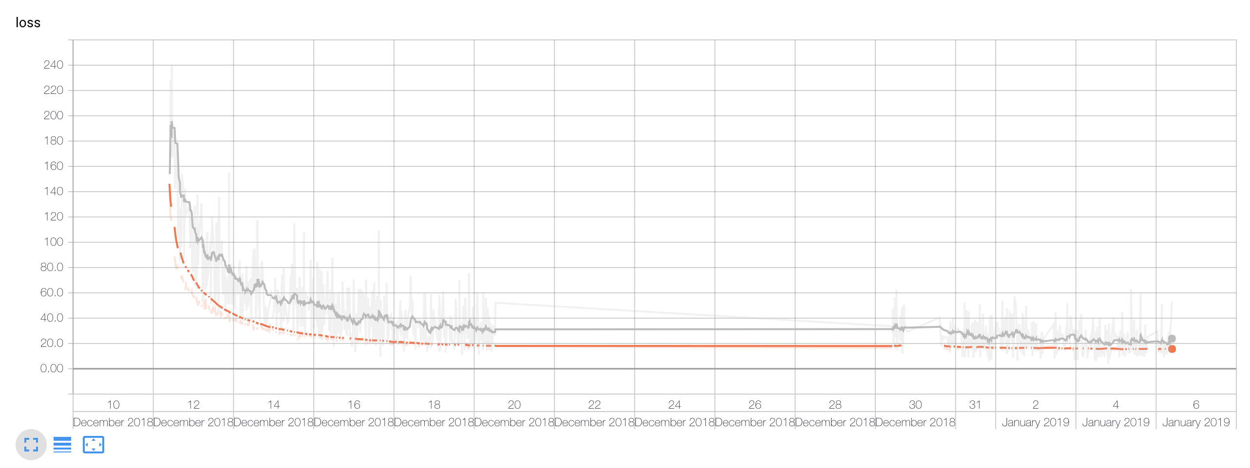
The statistics for the CTC Loss are included by default.
Here are the charts for the final model included in the GitHub repo:
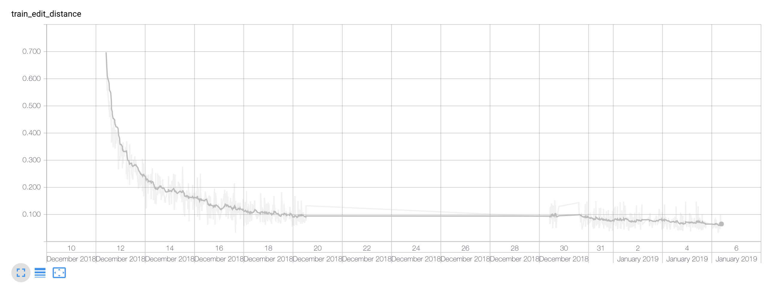
A thing to notice is that I paused the training between the 20th and 30th December.
The above chart presents the training time edit distance. Because of the pretty aggressive data augmentation, I noticed that throughout the whole process the training and validation edit distances didn’t differ hugely.
Following image shows the CTC loss with the orange line representing the evaluation runs.
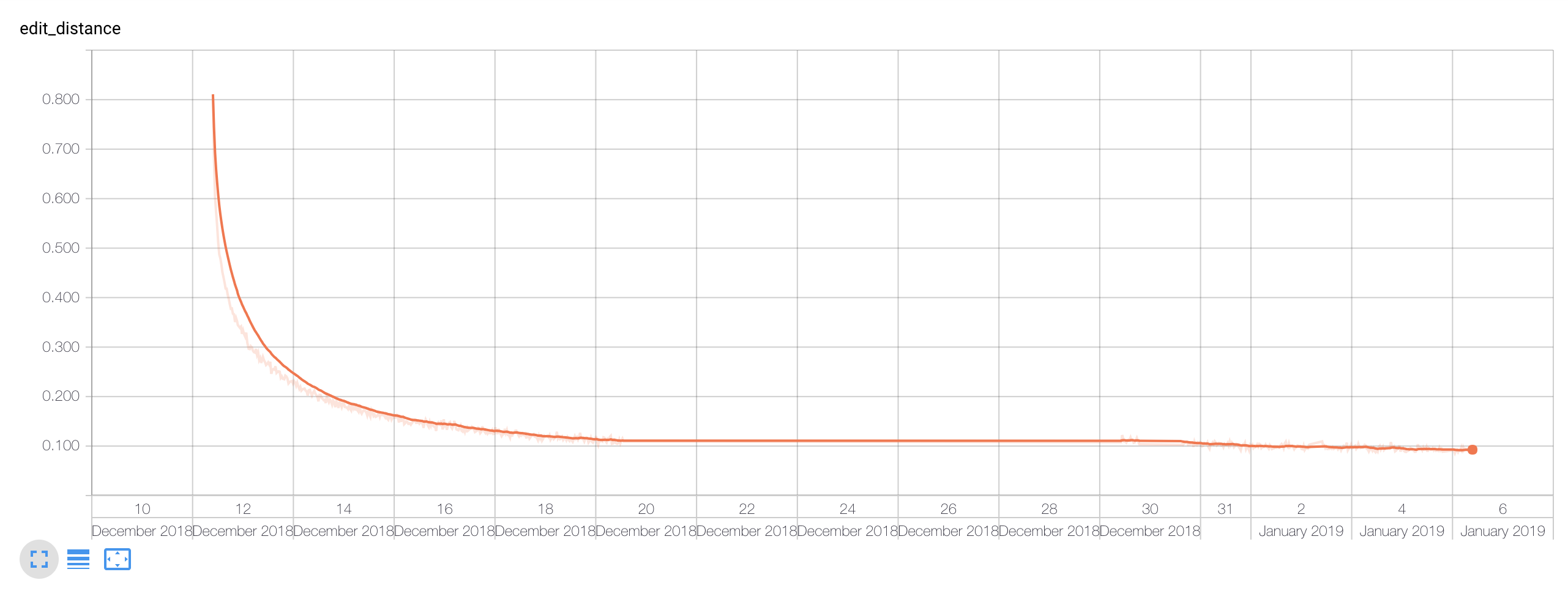
The evaluation edit distance is shown below. I stopped the training once the further gain for a whole day was dropping by less than 0.005.
Every machine learning model should be rigorously measured against meaningful accuracy statistics. Let’s see how we did:
test(
    dataset_params(
        batch_size=18,
        epochs=10,
        max_wave_length=320000,
        augment=True,
        random_noise=0.75,
        random_noise_factor_min=0.1,
        random_noise_factor_max=0.15,
        random_stretch_min=0.8,
        random_stretch_max=1.2
    ),
    codename='deep_max_20_seconds',
    alphabet=' !"&\',-.01234:;\\abcdefghijklmnopqrstuvwxyz', # !"&',-.01234:;\abcdefghijklmnopqrstuvwxyz
    causal_convolutions=False,
    stack_dilation_rates=[1, 3, 9, 27],
    stacks=6,
    stack_kernel_size=7,
    stack_filters=3*128,
    n_fft=160*8,
    frame_step=160*4,
    num_mel_bins=160,
    optimizer='Momentum',
    lr=0.00001,
    clip_gradients=20.0
)
The output:
(...)
INFO:tensorflow:Done running local_init_op.
INFO:tensorflow:Finished evaluation at 2019-01-07-10:51:09
INFO:tensorflow:Saving dict for global step 1525345: edit_distance = 0.07922124, global_step = 1525345, loss = 13.410753
(...)
This shows that for the test set, we’ve scored 0.079 in edit distance. We could invert it to call accuracy (somewhat naively though), which gives 92.1% — not too bad. The result would be officially reported as 7.9 LER.
What’s even nicer is the size of the model:
ls stats/causal_convolutions_False/codename_deep_max_20_seconds/frame_step_640/lower_edge_hertz_0/n_fft_1280/num_mel_bins_160/optimizer_Momentum/sampling_rate_16000/stack_dilation_rates_1_3_9_27/stack_filters_384/stack_kernel_size_7/stacks_6/upper_edge_hertz_8000/export/best_exporter/1546198558/variables -lh
total 204M
That’s 204MB for the model trained on the 375k+ dataset with aggressive augmentation (which makes the resulting dataset size effectively a couple times bigger).
It’s always nice to see what the results look like. Here’s the code that runs the model through the whole test sets and gathers the predicted transcriptions:
test_results = predict_test(
    codename='deep_max_20_seconds',
    alphabet=' !"&\',-.01234:;\\abcdefghijklmnopqrstuvwxyz', # !"&',-.01234:;\abcdefghijklmnopqrstuvwxyz
    causal_convolutions=False,
    stack_dilation_rates=[1, 3, 9, 27],
    stacks=6,
    stack_kernel_size=7,
    stack_filters=3*128,
    n_fft=160*8,
    frame_step=160*4,
    num_mel_bins=160,
    optimizer='Momentum',
    lr=0.00001,
    clip_gradients=20.0
)
[ b''.join(t['text']) for t in test_results ]
And the excerpt of the above is:
[b'without the dotaset the artice suistles',
 b"i've got to go to him",
 b'and you know it',
 b'down below in the darknes were hundrededs of people sleping in peace',
 b'strange images pased through my mind',
 b'the shep had taught him that',
 b'it was glaringly hot not a clou in hesky nor a breath of wind',
 b'your son went to serve at a distant place and became a cinturion',
 b'they made a boy continue tiging but he found nothing',
 b'the shoreas in da',
 b'fol the instructions here',
 b"the're caling to u not to give up and to kep on fighting",
 b'the shop was closed on monis',
 b'even coming down on the train together she wrote me',
 b"i'm going away he said",
 b"he wasn't asking for help",
 b'some of the grynsh was faling of the circular edge',
 b"i'd like to think",
 b'the alchemist robably already knew al that',
 b"you 'l take fiftly and like et",
 b'it was droping of in flakes and raining down on the sand',
 b"what's your name he asked",
 b"it's because you were not born",
 b'what do you think of that',
 b"if i had told tyo o you wouldn't have sen the pyramids",
 b"i havn't hert the baby complain yet",
 b'i told him wit could teach hr to ignore people who was had tend',
 b"the one you're blocking",
 b'henderson stod up with a spade in his hand',
 b"he didn't ned to sek out the old woman for this",
 b'only a minority of literature is reaten this way',
 b"i wish you wouldn't",
 ...]
Seems quite okay. You can immediately notice that some words are misspelled. This stems from the nature of the CTC algorithm itself. We’re predicting letters instead of words here. The good side is that the problem of out-of-vocabulary words is lessened. The worse part is that you’ll get e.g. ‘sek’ sometimes instead of ‘seek’. Because we’re outputting the logits for each example, it’s possible to use e.g. the CTCWordBeamSearch to constrain the output’s tokens to ones known within the corpus — making it predict the words instead.
Here’s the last little fun test: speech to text on the utterance I created on my laptop:
results = predict(
    'cv_corpus_v1/test-me.m4a',
    codename='deep_max_20_seconds',
    alphabet=' !"&\',-.01234:;\\abcdefghijklmnopqrstuvwxyz', # !"&',-.01234:;\abcdefghijklmnopqrstuvwxyz
    causal_convolutions=False,
    stack_dilation_rates=[1, 3, 9, 27],
    stacks=6,
    stack_kernel_size=7,
    stack_filters=3*128,
    n_fft=160*8,
    frame_step=160*4,
    num_mel_bins=160,
    optimizer='Momentum',
    lr=0.00001,
    clip_gradients=20.0
)
b''.join(results[0]['text'])
The result:
b'it semed to work just fine'Project on GitHub
The full Jupyter notebook’s code for this article can be found on GitHub: kamilc/speech-recognition.
The repository includes the bz2 archive of the best performing model I’ve trained. You can download it and run it as a web service via TensorFlow Serving, which we will cover in the next and last section here.
Serving the model with the TensorFlow Serving
The last step in this project is to serve our trained model as a web service. Thankfully, the TensorFlow project includes a ready to use “model server” that’s free to use: TensorFlow Serving.
The idea behind it is that we can run it, pointing it at the directory containing the models saved in the TensorFlow’s SavedModel format.
The deployment is extremely straightforward if you’re okay with running it from a Docker container. Let’s first pull the image:
docker pull tensorflow/servingNext, we need to download the saved model we’ve trained in this article from GitHub:
$ wget https://github.com/kamilc/speech-recognition/raw/master/best.tar.bz2
$ tar xvjf best.tar.bz2
In the next step, we need to start a container for the TensorFlow Serving image making it:
- open its port to outside
- mount the directory containing our model
- set the
MODEL_NAMEenvironment variable
As follows:
docker run -t --rm -p 8501:8501 -v "/home/kamil/projects/speech-recognition/best/1546646971:/models/speech/1" -e MODEL_NAME=speech tensorflow/servingThe service communicates via JSON payloads. Let’s prepare a payload.json file containing our request payload:
{"inputs": {"audio": <audio-data-here>, "length": <audio-raw-signal-length-here>}}We can now easily query the web service with the prepared request audio data:
curl -d @payload.json \
   -X POST http://localhost:8501/v1/models/speech:predict
Here’s what our intelligent web service responds with:
{
    "outputs": {
        "text": [
            [
                "c",
                "e",
                "v",
                "e",
                "r",
                "y",
                "t",
                "h",
                "i",
                "n",
                "g",
                " ",
                "i",
                "n",
                " ",
                "t",
                "h",
                "e",
                " ",
                "u",
                "n",
                "i",
                "v",
                "e",
                "r",
                "s",
                " ",
                "o",
                "v",
                "a",
                "l",
                "s",
                "h",
                "e",
                " ",
                "t",
                "e",
                "d",
                "i",
                "n",
                " ",
                "a",
                "w",
                "i",
                "t",
                " ",
                "j",
                "g",
                "m",
                "f",
                "t",
                "a",
                "r",
                "y",
                "s",
                "e"
            ]
        ],
        "logits": [
            [
                <logits-here>
            ]
        ]
    }
}
machine-learning python api audio
Comments