Recognizing handwritten digits: a quick peek into the basics of machine learning

By Kamil Ciemniewski
May 30, 2017
Previous in series:
- Learning from data basics: the Naive Bayes model
- Learning from data basics II: simple Bayesian Networks
In the previous two posts on machine learning, I presented a very basic introduction of an approach called “probabilistic graphical models”. In this post I’d like to take a tour of some different techniques while creating code that will recognize handwritten digits.
The handwritten digits recognition is an interesting topic that has been explored for many years. It is now considered one of the best ways to start the journey into the world of machine learning.
Taking the Kaggle challenge
We’ll take the “digits recognition” challenge as presented in Kaggle. It is an online platform with challenges for data scientists. Most of the challenges have their prizes expressed in real money to win. Some of them are there to help us out in our journey on learning data science techniques—so is the “digits recognition” contest.
The challenge
As explained on Kaggle:
MNIST (“Modified National Institute of Standards and Technology”) is the de facto “hello world” dataset of computer vision.
The “digits recognition” challenge is one of the best ways to get acquainted with machine learning and computer vision. The so-called “MNIST” dataset consists of 70k images of handwritten digits - each one grayscaled and of a 28x28 size. The Kaggle challenge is about taking a subset of 42k of them along with labels (what actual number does the image show) and “training” the computer on that set. The next step is to take the rest 28k of images without the labels and “predict” which actual number they present.
Here’s a short overview of how the digits in a set really look like (along with the numbers they represent):
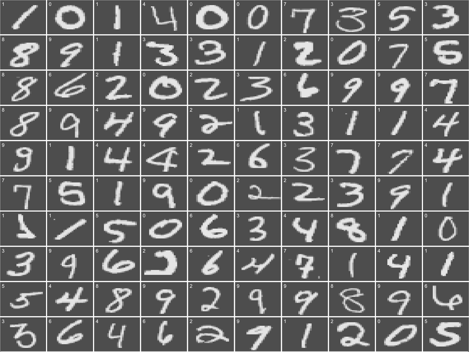
I have to admit that for some of them I have a really hard time recognizing the actual numbers on my own :)
The general approach to supervised learning
Learning from labelled data is what is called “supervised learning”. It’s supervised because we’re taking the computer by hand through the whole training data set and “teaching” it how the data that is linked with different labels “looks” like.
In all such scenarios we can express the data and labels as:
Y ~ X1, X2, X3, X4, ..., XnThe Y is called a dependent variable while each Xn are independent variables. This formula holds both for classification problems as well as regressions.
Classification is when the dependent variable Y is so called categorical—taking values from a concrete set without a meaningful order. Regression is when the Y is not categorical—most often continuous.
In the digits recognition challenge we’re faced with the classification task. The dependent variable takes values from the set:
Y = { 0, 1, 2, 3, 4, 5, 6, 7, 8, 9 }I’m sure the question you might be asking yourself now is: what are the independent variables Xn? It turns out to be the crux of the whole problem to solve :)
The plan of attack
A good introduction to computer vision techniques is a book by J. R Parker - “Algorithms for Image Processing and Computer Vision”. I encourage the reader to buy that book. I took some ideas from it while having fun with my own solution to the challenge.
The book outlines the ideas revolving around computing image profiles—for each side. For each row of pixels, a number representing the distance of the first pixel from the edge is computed. This way we’re getting our first independent variables. To capture even more information about digit shapes, we’ll also capture the differences between consecutive row values as well as their global maxima and minima. We’ll also compute the width of the shape for each row.
Because the handwritten digits vary greatly in their thickness, we will first preprocess the images to detect so-called skeletons of the digit. The skeleton is an image representation where the thickness of the shape has been reduced to just one.
Having the image thinned will also allow us to capture some more info about the shapes. We will write an algorithm that walks the skeleton and records the direction change frequencies.
Once we’ll have our set of independent variables Xn, we’ll use a classification algorithm to first learn in a supervised way (using the provided labels) and then to predict the values of the test data set. Lastly we’ll submit our predictions to Kaggle and see how well did we do.
Having fun with languages
In the data science world, the lingua franca still remains to be the R programming language. In the last years Python has also came close in popularity and nowadays we can say it’s the duo of R and Python that rule the data science world (not counting high performance code written e. g. in C++ in production systems).
Lately a new language designed with data scientists in mind has emerged - Julia. It’s a language with characteristics of both dynamically typed scripting languages as well as strictly typed compiled ones. It compiles its code into efficient native binary via LLVM—but it’s using it in a JIT fashion - inferring the types when needed on the go.
While having fun with the Kaggle challenge I’ll use Julia and Python for the so called feature extraction phase (the one in which we’re computing information about our Xn variables). I’ll then turn towards R for doing the classification itself. Note that I might use any of those languages at each step getting very similar results. The purpose of this series of articles is to be a bird eye fun overview so I decided that this way will be much more interesting.
Feature Extraction
The end result of this phase is the data frame saved as a CSV file so that we’ll be able to load it in R and do the classification.
First let’s define the general function in Julia that takes the name of the input CSV file and returns a data frame with features of given images extracted into columns:
using DataFrames

function get_data(name :: String, include_label = true)
  println("Loading CSV file into a data frame...")
  table = readtable(string(name, ".csv"))
  extract(table, include_label)
end
Now the extract function looks like the following:
"""
Extracts the features from the dataframe. Puts them into
separate columns and removes all other columns except the
labels.

The features:

* Left and right profiles (after fitting into the same sized rect):
  * Min
  * Max
  * Width[y]
  * Diff[y]
* Paths:
  * Frequencies of movement directions
  * Simplified directions:
    * Frequencies of 3 element simplified paths
"""
function extract(frame :: DataFrame, include_label = true)
  println("Reshaping data...")

  function to_image(flat :: Array{Float64}) :: Array{Float64}
    dim      = Base.isqrt(length(flat))
    reshape(flat, (dim, dim))'
  end

  from = include_label ? 2 : 1
  frame[:pixels] = map((i) -> convert(Array{Float64}, frame[i, from:end]) |> to_image, 1:size(frame, 1))
  images = frame[:, :pixels] ./ 255
  data = Array{Array{Float64}}(length(images))

  @showprogress 1 "Computing features..." for i in 1:length(images)
    features = pixels_to_features(images[i])
    data[i] = features_to_row(features)
  end
  start_column = include_label ? [:label] : []
  columns = vcat(start_column, features_columns(images[1]))

  result = DataFrame()
  for c in columns
    result[c] = []
  end

  for i in 1:length(data)
    if include_label
      push!(result, vcat(frame[i, :label], data[i]))
    else
      push!(result, vcat([],               data[i]))
    end
  end

  result
end
A few nice things to notice here about Julia itself are:
- The function documentation is written in Markdown
- We can nest functions inside other functions
- The language is statically and strongly typed
- Types can be inferred from the context
- It is often desirable to provide the concrete types to improve performance (but that an advanced Julia related topic)
- Arrays are indexed from 1
- There’s the nice |> operator found e. g. In Elixir (which I absolutely love)
The above code converts the images to be arrays of Float64 and converts the values to be within 0 and 1 (instead of 0..255 originally).
A thing to notice is that in Julia we can vectorize operations easily and we’re using this fact to tersely convert our number:
images = frame[:, :pixels] ./ 255We are referencing the pixels_to_features function which we define as:
"""
Returns ImageFeatures struct for the image pixels
given as an argument
"""
function pixels_to_features(image :: Array{Float64})
  dim      = Base.isqrt(length(image))
  skeleton = compute_skeleton(image)
  bounds   = compute_bounds(skeleton)
  resized  = compute_resized(skeleton, bounds, (dim, dim))
  left     = compute_profile(resized, :left)
  right    = compute_profile(resized, :right)
  width_min, width_max, width_at = compute_widths(left, right, image)
  frequencies, simples = compute_transitions(skeleton)

  ImageStats(dim, left, right, width_min, width_max, width_at, frequencies, simples)
end
This in turn uses the ImageStats structure:
immutable ImageStats
  image_dim             :: Int64
  left                  :: ProfileStats
  right                 :: ProfileStats
  width_min             :: Int64
  width_max             :: Int64
  width_at              :: Array{Int64}
  direction_frequencies :: Array{Float64}

  # The following adds information about transitions
  # in 2 element simplified paths:
  simple_direction_frequencies :: Array{Float64}
end

immutable ProfileStats
  min :: Int64
  max :: Int64
  at  :: Array{Int64}
  diff :: Array{Int64}
end
The pixels_to_features function first gets the skeleton of the digit shape as an image and then uses other functions passing that skeleton to them. The function returning the skeleton utilizes the fact that in Julia it’s trivially easy to use Python libraries. Here’s its definition:
using PyCall

@pyimport skimage.morphology as cv

"""
Thin the number in the image by computing the skeleton
"""
function compute_skeleton(number_image :: Array{Float64}) :: Array{Float64}
  convert(Array{Float64}, cv.skeletonize_3d(number_image))
end
It uses the scikit-image library’s function skeletonize3d by using the @pyimport macro and using the function as if it was just a regular Julia code.
Next the code crops the digit itself from the 28x28 image and resizes it back to 28x28 so that the edges of the shape always “touch” the edges of the image. For this we need the function that returns the bounds of the shape so that it’s easy to do the cropping:
function compute_bounds(number_image :: Array{Float64}) :: Bounds
  rows = size(number_image, 1)
  cols = size(number_image, 2)

  saw_top = false
  saw_bottom = false

  top = 1
  bottom = rows
  left = cols
  right = 1

  for y = 1:rows
    saw_left = false
    row_sum = 0

    for x = 1:cols
      row_sum += number_image[y, x]

      if !saw_top && number_image[y, x] > 0
        saw_top = true
        top = y
      end

      if !saw_left && number_image[y, x] > 0 && x < left
        saw_left = true
        left = x
      end

      if saw_top && !saw_bottom && x == cols && row_sum == 0
        saw_bottom = true
        bottom = y - 1
      end

      if number_image[y, x] > 0 && x > right
        right = x
      end
    end
  end
  Bounds(top, right, bottom, left)
end
Resizing the image is pretty straight-forward:
using Images

function compute_resized(image :: Array{Float64}, bounds :: Bounds, dims :: Tuple{Int64, Int64}) :: Array{Float64}
  cropped = image[bounds.left:bounds.right, bounds.top:bounds.bottom]
  imresize(cropped, dims)
end
Next, we need to compute the profile stats as described in our plan of attack:
function compute_profile(image :: Array{Float64}, side :: Symbol) :: ProfileStats
  @assert side == :left || side == :right

  rows = size(image, 1)
  cols = size(image, 2)

  columns = side == :left ? collect(1:cols) : (collect(1:cols) |> reverse)
  at = zeros(Int64, rows)
  diff = zeros(Int64, rows)
  min = rows
  max = 0

  min_val = cols
  max_val = 0

  for y = 1:rows
    for x = columns
      if image[y, x] > 0
        at[y] = side == :left ? x : cols - x + 1

        if at[y] < min_val
          min_val = at[y]
          min = y
        end

        if at[y] > max_val
          max_val = at[y]
          max = y
        end
        break
      end
    end
    if y == 1
      diff[y] = at[y]
    else
      diff[y] = at[y] - at[y - 1]
    end
  end

  ProfileStats(min, max, at, diff)
end
The widths of shapes can be computed with the following:
function compute_widths(left :: ProfileStats, right :: ProfileStats, image :: Array{Float64}) :: Tuple{Int64, Int64, Array{Int64}}
  image_width = size(image, 2)
  min_width = image_width
  max_width = 0
  width_ats = length(left.at) |> zeros

  for row in 1:length(left.at)
    width_ats[row] = image_width - (left.at[row] - 1) - (right.at[row] - 1)

    if width_ats[row] < min_width
      min_width = width_ats[row]
    end

    if width_ats[row] > max_width
      max_width = width_ats[row]
    end
  end

  (min_width, max_width, width_ats)
end
And lastly, the transitions:
function compute_transitions(image :: Image) :: Tuple{Array{Float64}, Array{Float64}}
  history = zeros((size(image,1), size(image,2)))

  function next_point() :: Nullable{Point}
    point = Nullable()

    for row in 1:size(image, 1) |> reverse
      for col in 1:size(image, 2) |> reverse
        if image[row, col] > 0.0 && history[row, col] == 0.0
          point = Nullable((row, col))
          history[row, col] = 1.0

          return point
        end
      end
    end
  end

  function next_point(point :: Nullable{Point}) :: Tuple{Nullable{Point}, Int64}
    result = Nullable()
    trans = 0

    function direction_to_moves(direction :: Int64) :: Tuple{Int64, Int64}
      # for frequencies:
      # 8 1 2
      # 7 - 3
      # 6 5 4
      [
       ( -1,  0 ),
       ( -1,  1 ),
       (  0,  1 ),
       (  1,  1 ),
       (  1,  0 ),
       (  1, -1 ),
       (  0, -1 ),
       ( -1, -1 ),
      ][direction]
    end

    function peek_point(direction :: Int64) :: Nullable{Point}
      actual_current = get(point)

      row_move, col_move = direction_to_moves(direction)

      new_row = actual_current[1] + row_move
      new_col = actual_current[2] + col_move

      if new_row <= size(image, 1) && new_col <= size(image, 2) &&
         new_row >= 1 && new_col >= 1
        return Nullable((new_row, new_col))
      else
        return Nullable()
      end
    end

    for direction in 1:8
      peeked = peek_point(direction)

      if !isnull(peeked)
        actual = get(peeked)
        if image[actual[1], actual[2]] > 0.0 && history[actual[1], actual[2]] == 0.0
          result = peeked
          history[actual[1], actual[2]] = 1
          trans = direction
          break
        end
      end
    end

    ( result, trans )
  end

  function trans_to_simples(transition :: Int64) :: Array{Int64}
    # for frequencies:
    # 8 1 2
    # 7 - 3
    # 6 5 4

    # for simples:
    # - 1 -
    # 4 - 2
    # - 3 -
    [
      [ 1 ],
      [ 1, 2 ],
      [ 2 ],
      [ 2, 3 ],
      [ 3 ],
      [ 3, 4 ],
      [ 4 ],
      [ 1, 4 ]
    ][transition]
  end

  transitions     = zeros(8)
  simples         = zeros(16)
  last_simples    = [ ]
  point           = next_point()
  num_transitions = .0
  ind(r, c) = (c - 1)*4 + r

  while !isnull(point)
    point, trans = next_point(point)

    if isnull(point)
      point = next_point()
    else
      current_simples = trans_to_simples(trans)
      transitions[trans] += 1
      for simple in current_simples
        for last_simple in last_simples
          simples[ind(last_simple, simple)] +=1
        end
      end
      last_simples = current_simples
      num_transitions += 1.0
    end
  end

  (transitions ./ num_transitions, simples ./ num_transitions)
end
All those gathered features can be turned into rows with:
function features_to_row(features :: ImageStats)
  lefts       = [ features.left.min,  features.left.max  ]
  rights      = [ features.right.min, features.right.max ]

  left_ats    = [ features.left.at[i]  for i in 1:features.image_dim ]
  left_diffs  = [ features.left.diff[i]  for i in 1:features.image_dim ]
  right_ats   = [ features.right.at[i] for i in 1:features.image_dim ]
  right_diffs = [ features.right.diff[i]  for i in 1:features.image_dim ]
  frequencies = features.direction_frequencies
  simples     = features.simple_direction_frequencies

  vcat(lefts, left_ats, left_diffs, rights, right_ats, right_diffs, frequencies, simples)
end
Similarly we can construct the column names with:
function features_columns(image :: Array{Float64})
  image_dim   = Base.isqrt(length(image))

  lefts       = [ :left_min,  :left_max  ]
  rights      = [ :right_min, :right_max ]

  left_ats    = [ Symbol("left_at_",  i) for i in 1:image_dim ]
  left_diffs  = [ Symbol("left_diff_",  i) for i in 1:image_dim ]
  right_ats   = [ Symbol("right_at_", i) for i in 1:image_dim ]
  right_diffs = [ Symbol("right_diff_", i) for i in 1:image_dim ]
  frequencies = [ Symbol("direction_freq_", i)   for i in 1:8 ]
  simples     = [ Symbol("simple_trans_", i)   for i in 1:4^2 ]

  vcat(lefts, left_ats, left_diffs, rights, right_ats, right_diffs, frequencies, simples)
end
The data frame constructed with the get_data function can be easily dumped into the CSV file with the writeable function from the DataFrames package.
You can notice that gathering / extracting features is a lot of work. All this was needed to be done because in this article we’re focusing on the somewhat “classical" way of doing machine learning. You might have heard about algorithms existing that mimic how the human brain learns. We’re not focusing on them here. This we will explore in some future article.
We use the mentioned writetable on data frames computed for both training and test datasets to store two files: processed_train.csv and processed_test.csv.
Choosing the model
For the task of classifying I decided to use the XGBoost library which is somewhat a hot new technology in the world of machine learning. It’s an improvement over the so-called Random Forest algorithm. The reader can read more about XGBoost on its website: https://xgboost.readthedocs.io/.
Both random forest and xgboost revolve around the idea called ensemble learning. In this approach we’re not getting just one learning model—the algorithm actually creates many variations of models and uses them to collectively come up with better results. This is as much as can be written as a short description as this article is already quite lengthy.
Training the model
The training and classification code in R is very simple. We first need to load the libraries that will allow us to load data as well as to build the classification model:
library(xgboost)
library(readr)
Loading the data into data frames is equally straight-forward:
processed_train <- read_csv("processed_train.csv")
processed_test <- read_csv("processed_test.csv")
We then move on to preparing the vector of labels for each row as well as the matrix of features:
labels = processed_train$label
features = processed_train[, 2:141]
features = scale(features)
features = as.matrix(features)
The train-test split
When working with models, one of the ways of evaluating their performance is to split the data into so-called train and test sets. We train the model on one set and then we predict the values from the test set. We then calculate the accuracy of predicted values as the ratio between the number of correct predictions and the number of all observations.
Because Kaggle provides the test set without labels, for the sake of evaluating the model’s performance without the need to submit the results, we’ll split our Kaggle-training set into local train and test ones. We’ll use the amazing caret library which provides a wealth of tools for doing machine learning:
library(caret)

index <- createDataPartition(processed_train$label, p = .8,
                             list = FALSE,
                             times = 1)

train_labels <- labels[index]
train_features <- features[index,]

test_labels <- labels[-index]
test_features <- features[-index,]
The above code splits the set uniformly based on the labels so that the train set is approximately 80% in size of the whole data set.
Using XGBoost as the classification model
We can now make our data digestible by the XGBoost library:
train <- xgb.DMatrix(as.matrix(train_features), label = train_labels)
test  <- xgb.DMatrix(as.matrix(test_features),  label = test_labels)
The next step is to make the XGBoost learn from our data. The actual parameters and their explanations are beyond the scope of this overview article, but the reader can look them up on the XGBoost pages:
model <- xgboost(train,
                 max_depth = 16,
                 nrounds = 600,
                 eta = 0.2,
                 objective = "multi:softmax",
                 num_class = 10)
It’s critically important to pass the objective as “multi:softmax" and num_class as 10.
Simple performance evaluation with confusion matrix
After waiting a while (couple of minutes) for the last batch of code to finish computing, we now have the classification model ready to be used. Let’s use it to predict the labels from our test set:
predicted = predict(model, test)This returns the vector of predicted values. We’d now like to check how well our model predicts the values. One of the easiest ways is to use the so-called confusion matrix.
As per Wikipedia, confusion matrix is simply:
(…) also known as an error matrix, is a specific table layout that allows visualization of the performance of an algorithm, typically a supervised learning one (in unsupervised learning it is usually called a matching matrix). Each column of the matrix represents the instances in a predicted class while each row represents the instances in an actual class (or vice versa). The name stems from the fact that it makes it easy to see if the system is confusing two classes (i.e. commonly mislabelling one as another).
The caret library provides a very easy to use function for examining the confusion matrix and statistics derived from it:
confusionMatrix(data=predicted, reference=labels)The function returns an R list that gets pretty printed to the R console. In our case it looks like the following:
Confusion Matrix and Statistics

          Reference
Prediction   0   1   2   3   4   5   6   7   8   9
         0 819   0   3   3   1   1   2   1  10   5
         1   0 923   0   4   5   1   5   3   4   5
         2   4   2 766  26   2   6   8  12   5   0
         3   2   0  15 799   0  22   2   8   0   8
         4   5   2   1   0 761   1   0  15   4  19
         5   1   3   0  13   2 719   3   0   9   6
         6   5   3   4   1   6   5 790   0  16   2
         7   1   7  12   9   2   3   1 813   4  16
         8   6   2   4   7   8  11   8   5 767  10
         9   5   2   1  13  22   6   1  14  14 746

Overall Statistics

               Accuracy : 0.9411
                 95% CI : (0.9358, 0.946)
    No Information Rate : 0.1124
    P-Value [Acc > NIR] : < 2.2e-16

                  Kappa : 0.9345
 Mcnemar's Test P-Value : NA

(...)
Each column in the matrix represents actual labels while rows represent what our algorithms predicted this value to be. There’s also the accuracy rate printed for us and in this case it equals 0.9411. This means that our code was able to predict correct values of handwritten digits for 94.11% of observations.
Submitting the results
We got 0.9411 of an accuracy rate for our local test set and it turned out to be very close to the one we got against the test set coming from Kaggle. After predicting the competition values and submitting them, the accuracy rate computed by Kaggle was 0.94357. That’s quite okay given the fact that we’re not using here any of the new and fancy techniques.
Also, we haven’t done any parameter tuning which could surely improve the overall accuracy. We could also revisit the code from the features extraction phase. One improvement I can think of would be to first crop and resize back - and only then compute the skeleton which might preserve more information about the shape. We could also use the confusion matrix and taking the number that was being confused the most, look at the real images that we failed to recognize. This could lead us to conclusions about improvements to our feature extraction code. There’s always a way to extract more information.
Nowadays, Kagglers from around the world were successfully using advanced techniques like Convolutional Neural Networks getting accuracy scores close to 0.999. Those live in somewhat different branch of the machine learning world though. Using this type of neural networks we don’t need to do the feature extraction on our own. The algorithm includes the step that automatically gathers features that it later on feeds into the network itself. We will take a look at them in some of the future articles.
Comments