Our Blog

Learning from data basics II: simple Bayesian Networks

By Kamil Ciemniewski
April 12, 2016

In my last article I presented an approach that simplifies computations of very complex probability models. It makes these complex models viable by shrinking the amount of needed memory and improving the speed of computing probabilities. The approach we were exploring is called the Naive Bayes model.

The context was the e-commerce feature in which a user is presented with the promotion box. The box shows the product category the user is most likely to buy.

Though the results we got were quite good, I promised to present an approach that gives much better ones. While the Naive Bayes approach may not be acceptable in some scenarios due to the gap between approximated and real values, the approach presented in this article will make this distance much, much smaller.

Naive Bayes as a simple Bayesian Network

When exploring the Naive Bayes model, we said that there is a probabilistic assumption the model makes in order to simplify the computations. In the last article I wrote:

The Naive Bayes assumption says that the distribution factorizes the way we did it only if the features are conditionally independent given the category.

Expressing variable dependencies as a graph

Let’s imagine the visual representation of the relations between the random variables in the Naive Bayes model. Let’s make it into a directed acyclic graph. Let’s mark the dependence of one variable on another as a graph edge from the parent node pointing to it’s dependent node.

Because of the assumption the Naive Bayes model enforces, its structure as a graph looks like the following:

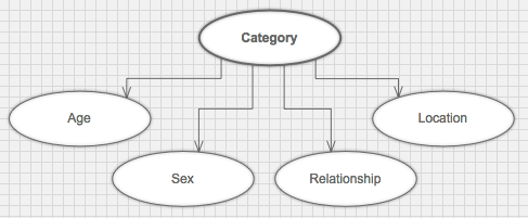
You can notice there are no lines between all the “evidence” nodes. The assumption says that knowing the category, we have all needed knowledge about every single evidence node. This makes category the parent of all the other nodes. Intuitively, we can say that knowing the class (in this example, the category) we know everything about all features. It’s easy to notice that this assumption doesn’t hold in this example.

In our fake data generator, we made it so that e.g. relationship status depends on age. We’ve also made the category depend on sex and age directly. This way we can’t say that knowing category we know everything about e. g. age. The random variables age and sex are not independent even if we know the value of category. It is clear that the above graph does not model the dependency relationships between these random variables.

Let’s draw a graph that represents our fake data model better:

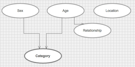
The combination of a graph like the one above and the probability distribution that follows the independencies it describes are known as a Bayesian Network.

Using the graph representation in practice - the chain rule for Bayesian Networks

The fact that our distribution is part of the Bayesian Network, allows us to use the formula for simplifying the distribution itself. The formula is called the chain rule for Bayesian Networks and for our particular example looks like the following:

p(cat, sex, age, rel, loc) = p(sex) * p(age) * p(loc) * p(rel | age) * p(cat | sex, age)

You can notice that the equation is just a product of a number of factors. There’s one factor for each random variable. The factors for variables that in the graph don’t have any parents are expressed as p(var) while those that do are expressed as p(var | par) or p(var | par1, par2…).

Notice that the Naive Bayes model fits perfectly into this equation. If you were to take the first graph presented in this article—​for the Naive Bayes, and use the above equation, you’d get exactly the formula we used in the last article.

Coding the updated probabilistic model

Before going further, I strongly advise you to make sure you read the previous article - about the Naive Bayes model - to fully understand the classes used in the code in this section.

Let’s take our chain rule equation and simplify it:

p(cat, sex, age, rel, loc) = p(sex) * p(age) * p(loc) * p(rel | age) * p(cat | sex, age)

Again a conditional distrubution can be expressed as:

p(a | b) = p(a, b) / p(b)

This gives us:

p(cat, sex, age, rel, loc) = p(sex) * p(age) * p(loc) * (p(rel, age)/ p(age)) * (p(cat, sex, age) / p(sex, age))

We can easily factor out the p(age) with:

p(cat, sex, age, rel, loc) = p(sex) * p(loc) * p(rel, age) * (p(cat, sex, age) / p(sex, age))

Let’s define needed random variables and factors:

category = RandomVariable.new :category, [ :veggies, :snacks, :meat, :drinks, :beauty, :magazines ]
age      = RandomVariable.new :age,      [ :teens, :young_adults, :adults, :elders ]
sex      = RandomVariable.new :sex,      [ :male, :female ]
relation = RandomVariable.new :relation, [ :single, :in_relationship ]
location = RandomVariable.new :location, [ :us, :canada, :europe, :asia ]

loc_dist     = Factor.new [ location ]
sex_dist     = Factor.new [ sex ]
rel_age_dist = Factor.new [ relation, age ]
cat_age_sex_dist = Factor.new [ category, age, sex ]
age_sex_dist = Factor.new [ age, sex ]

full_dist = Factor.new [ category, age, sex, relation, location ]

The learning part is as trivial as in the Naive Bayes case. The only difference is the set of distributions involved:

Model.generate(1000).each do |user|
  user.baskets.each do |basket|
    basket.line_items.each do |item|
      loc_dist.observe! location: user.location
      sex_dist.observe! sex: user.sex
      rel_age_dist.observe! relation: user.relationship, age: user.age
      cat_age_sex_dist.observe! category: item.category, age: user.age, sex: user.sex
      age_sex_dist.observe! age: user.age, sex: user.sex
      full_dist.observe! category: item.category, age: user.age, sex: user.sex,
        relation: user.relationship, location: user.location
    end
  end
end

The inference part is also very similar to the one from the previous article. Here too the only difference are the distributions involved:

infer = -> (age, sex, rel, loc) do
  all = category.values.map do |cat|
    pl  = loc_dist.value_for location: loc
    ps  = sex_dist.value_for sex: sex
    pra = rel_age_dist.value_for relation: rel, age: age
    pcas = cat_age_sex_dist.value_for category: cat, age: age, sex: sex
    pas = age_sex_dist.value_for age: age, sex: sex
    { category: cat, value: (pl * ps * pra * pcas) / pas }
  end

  all_full = category.values.map do |cat|
    val = full_dist.value_for category: cat, age: age, sex: sex,
            relation: rel, location: loc
    { category: cat, value: val }
  end

  win      = all.max      { |a, b| a[:value] <=> b[:value] }
  win_full = all_full.max { |a, b| a[:value] <=> b[:value] }

  puts "Best match for #{[ age, sex, rel, loc ]}:"
  puts "   #{win[:category]} => #{win[:value]}"
  puts "Full pointed at:"
  puts "   #{win_full[:category]} => #{win_full[:value]}\n\n"
end

The results

Now let’s run the inference procedure with the same set of examples as in the previous post to compare the results:

infer.call :teens, :male, :single, :us
infer.call :young_adults, :male, :single, :asia
infer.call :adults, :female, :in_relationship, :europe
infer.call :elders, :female, :in_relationship, :canada

Which yields:

Best match for [:teens, :male, :single, :us]:
   snacks => 0.020610837341908994
Full pointed at:
   snacks => 0.02103999999999992

Best match for [:young_adults, :male, :single, :asia]:
   meat => 0.001801062449999991
Full pointed at:
   meat => 0.0010700000000000121

Best match for [:adults, :female, :in_relationship, :europe]:
   beauty => 0.0007693377820183494
Full pointed at:
   beauty => 0.0008300000000000074

Best match for [:elders, :female, :in_relationship, :canada]:
   veggies => 0.0024346445741176875
Full pointed at:
   veggies => 0.0034199999999999886

Just as with using the Naive Bayes, we got correct values for all cases. When you look closer though, you can notice that the resulting probability values were much closer to the original, full distribution ones. The approach we took here makes the values differ only a couple times in 10000. That result could make a difference in the e-commerce shop from the example if it were visited by millions of customers each month.

machine-learning optimization probability ruby