Our Blog

How to use dependent dropdowns in Microsoft Excel

By Nicholas Piano
August 2, 2023

Dropdowns are a way to constrain the input of a cell to a set of values. This can be useful for data validation, or for making a spreadsheet more user-friendly. In this article, we will look at how to create two types of dropdowns in Microsoft Excel: the basic dropdown and the dependent dropdown.

Using this, we can expand to more complex dropdown dependencies and spreadsheet generation, including validation using the Axlsx gem in Ruby.

The basic dropdown

A dropdown takes its data from a list of values specified by a range. This could be a range of cells, or a named range. To create a dropdown, first select the cell you want to add the dropdown to. Then, go to the Data tab, and click on Data Validation.

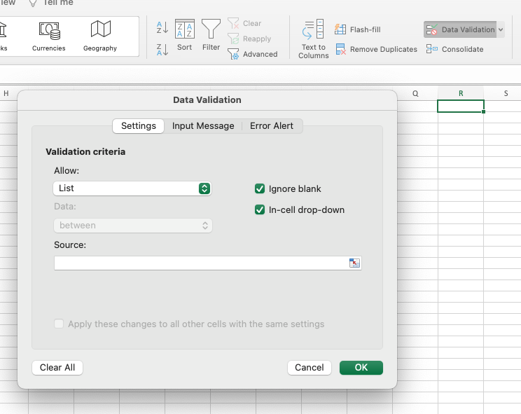
Data Validation Menu

Specify the range, e.g. =Sheet1!$A$1:$A$5. Then, select the “List” option under “Allow”. You can also specify an input message and error message, which will be displayed when the user selects the cell. Note that the range can come from another worksheet.

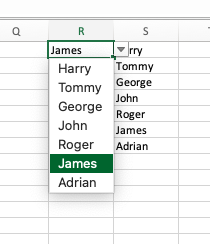
Basic Range

And that’s it! You can now constrain the input of the cell to the values in the range.

The dependent dropdown

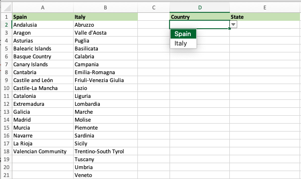
Things get a little more complicated when we want to create a dropdown that depends on another dropdown. For example, we might want to have a dropdown for “Country”, and another dropdown for “State”, where the list of states depends on the country selected.

To do this, the associations between countries and states must be stored in a way that can be easily accessed by Excel. For example:

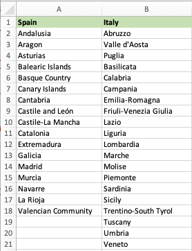
Given this data, the source for the “Country” dropdown will be =Sheet1!$A$1:$B$1. If our country dropdown is in cell D1, the source for the “State” dropdown will be =INDIRECT($D$1). Note that the INDIRECT function is used to convert the string into a reference to the range. That is, the string in the target cell is interpreted as a range or reference. The & operator is used to concatenate the string with the cell reference.

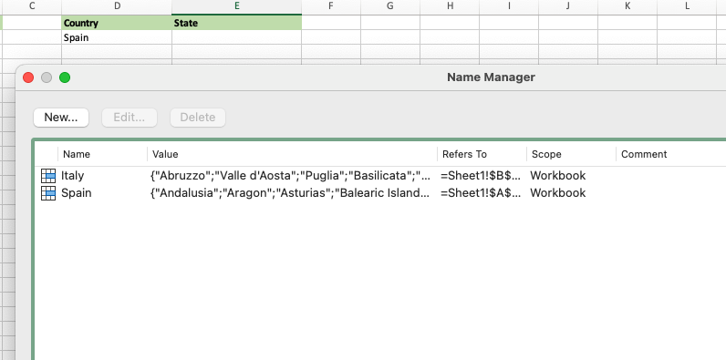
There is one more element needed to make this work: the named range. The value of $D$1 in this case will simply be the value “Spain” or “Italy”, which does not, by itself, refer to a range. However, we can create a named range that refers to the range of states for each country. For example, we can create a named range called “Spain” that refers to =Sheet1!$B$2:$B$4, and a named range called “Italy” that refers to =Sheet1!$B$5:$B$7. Then, the value of $D$1 will be interpreted as a reference to the named range, and the dropdown will be populated with the correct values.

To do this, go to the Formulas tab, and click on Name Manager. Then, click on New, and enter the name and the range. Repeat this for each country. In the end, the name manager should look like this:

Using the Axlsx gem in Ruby

Now that we’ve seen how to create dependent dropdowns in Excel manually, we can use this to create more complex spreadsheets using scripts. We can use the Axlsx gem in Ruby to generate spreadsheets that include the same dropdowns and data validation as before, but now generated automatically from available data.

Let’s recreate our example above using axlsx. First, we need to create a workbook and a worksheet:

require 'axlsx'

# first, let's add the data
spain_regions = ['Andalusia', 'Aragon', 'Asturias', 'Balearic Islands', 'Basque Country', 'Canary Islands', 'Cantabria', 'Castile and Leon', 'Castile-La Mancha', 'Catalonia', 'Ceuta', 'Extremadura', 'Galicia', 'La Rioja', 'Madrid', 'Melilla', 'Murcia', 'Navarre', 'Valencian Community']
italy_regions = ['Abruzzo', 'Aosta Valley', 'Apulia', 'Basilicata', 'Calabria', 'Campania', 'Emilia-Romagna', 'Friuli-Venezia Giulia', 'Lazio', 'Liguria', 'Lombardy', 'Marche', 'Molise', 'Piedmont', 'Sardinia', 'Sicily', 'Trentino-South Tyrol', 'Tuscany', 'Umbria', 'Veneto']

p = Axlsx::Package.new
wb = p.workbook

# In order to demonstrate how to make references to other sheets in the revelant
# formulas, we will create two sheets, one for the data and one for the dropdowns.
wb.add_worksheet(name: 'Countries and Regions') do |sheet|
    headers = ['Spain', 'Italy']
    sheet.add_row(headers)

    # The data will be organised into two columns for easy access.
    # We will use the zip method to iterate over both arrays at the same time.
    spain_regions.zip(italy_regions).each do |spain_region, italy_region|
        sheet.add_row([spain_region, italy_region])
    end

    # The three ranges we will use are:
    # - The range of countries (the headers), which will be used for the first dropdown.
    # - The range of regions (two ranges) for each country, which will be used for the second dropdown.
end

wb.add_worksheet(name: 'Dropdowns') do |sheet|
    # The first dropdown will be in cell D1.
    sheet.add_data_validation('D1', {
        :type => :list,
        :hideDropDown => false,
        :formula1 => "='Countries and Regions'!$A$1:$B$1",
        :prompt => 'Select a country',
        :showErrorMessage => true,
        :errorTitle => 'Invalid Country',
        :error => 'Please select a valid country.',
        :errorStyle => :stop,
        :showInputMessage => true,
    })

    # The second dropdown will be in cell D2.
    # Note the INDIRECT function that uses the value of D1 to determine the range.
    # This will reference the named range for the selected country.
    sheet.add_data_validation('D2', {
        type: :list,
        formula1: "INDIRECT($D$1)",
        allow_blank: true,
        show_input_message: true,
        show_error_message: true,
        error_title: 'Invalid Region',
        error_message: 'Please select a valid region.',
        error_style: :stop,
        show_drop_down: true
    })
end

# Lastly, add the named ranges for each country
spain_end_row = spain_regions.length + 1
wb.add_defined_name("'Countries and Regions'!$A$2:$A$#{spain_end_row}", { :name => "Spain" })

italy_end_row = italy_regions.length + 1
wb.add_defined_name("'Countries and Regions'!$B$2:$B$#{italy_end_row}", { :name => "Italy" })

# Note that we have accounted for the length of the array when creating the named range.

This script should do everything we need to create the spreadsheet. The only thing left to do is to save it:

p.serialize('dropdowns.xlsx')

And that’s it! You can now generate a template complete with complex data validation and dropdowns.

Conclusion

Excel spreadsheets are a powerful tool for data analysis and visualisation. They are extremely portable, allowing them to be used as templates for data collection, such as polls.

In order to gather high quality data, it is important to ensure that the data is entered correctly. One way to do this is to use dropdowns and data validation.

In this article, we have seen how to create dependent dropdowns in Excel, and how to use the Axlsx gem in Ruby to generate spreadsheets with dropdowns and data validation.

One limitation to be aware of: while most spreadsheet functionality is common between different spreadsheet software, data validation and dropdowns are not. This means that the spreadsheets generated by the Axlsx gem will only work in Excel, and not in other spreadsheet software such as LibreOffice Calc.

With that, you can take your data collection to the next level!

tips ruby